Data description
The dataset used in this analysis is sourced from the Bureau van Dijk OSIRIS database, a globally recognised repository of harmonised financial information covering publicly listed and major private firms (Bureau van Dijk, 2025). For this project, firm-level financial data were extracted for German companies across the 2018–2021 accounting years, capturing both pre-pandemic conditions and the period most directly affected by COVID-19.
Each observation represents a firm’s reported financial position for a given accounting year, enabling longitudinal analysis of changes in profitability, liquidity, leverage, and overall financial resilience over time. The following sections document the reproducible process used to load, combine, standardise, and prepare the raw OSIRIS extracts for analysis.
Loading the data
This is the library used for this data.
Show code
library(dplyr)
library(stringr)
library(janitor)
library(skimr)
library(tsibble)
library(knitr)
library(naniar)
library(patchwork)
library(plotly)
library(tsibbletalk)
library(feasts)
library(broom)
library(purrr)
library(cassowaryr)
library(gganimate)
library(gifski)
library(kableExtra)
library(ggplot2)
library(scales)
library(tidyr)
library(ggrepel)
library(viridisLite)
The following code loads the annual OSIRIS extracts for Germany and stores each year’s data as a separate object, preserving the original reporting structure while enabling systematic combination.
Show code
#define the folder
data_directory <- "osiris"

#filter only germany
germany_file_paths <- list.files(
  data_directory,
  pattern = "^osiris_?Germany_(2018|2019|2020|2021)\\.rda$",
  full.names = TRUE,
  ignore.case = TRUE
)

#name the list by file stems
germany_file_stems <- tools::file_path_sans_ext(basename(germany_file_paths))
osiris_germany <- setNames(vector("list", length(germany_file_paths)), germany_file_stems)

#load each file
for (file_index in seq_along(germany_file_paths)) {
  temporary_environment <- new.env(parent = emptyenv())
  load(germany_file_paths[file_index], envir = temporary_environment)
  loaded_objects <- as.list(temporary_environment)

  #If the file holds one object, store that object; otherwise store the sub-list
  osiris_germany[[file_index]] <- if (length(loaded_objects) == 1) loaded_objects[[1]] else loaded_objects
}
Combining the data
Once loaded, the annual datasets are combined into a single longitudinal data frame. A reporting year variable is extracted from each file name to facilitate temporal ordering and year-to-year comparison.
Show code
#build a single data frame with a 'year' column taken from the filename
combined_germany <- {
  germany_parts <- vector("list", length(osiris_germany))
  names(germany_parts) <- names(osiris_germany)

  for (file_stem in names(osiris_germany)) {
    data_frame_from_file <- osiris_germany[[file_stem]]
    extracted_year <- as.integer(str_extract(file_stem, "\\d{4}"))

    germany_parts[[file_stem]] <- mutate(data_frame_from_file, year = extracted_year)
  }

  #bind and sort by year (optional)
  bind_rows(germany_parts) |>
    arrange(year)
}
Data cleaning & standardisation
After combining the annual extracts, the dataset is transformed into an analysis-ready format. This step standardises column names, maps vendor-specific field labels to clearly defined analytical variables, and constructs a fiscal-year indicator based on reported year-end dates.
Only firm identifiers, industry classifications, and financial variables relevant to the analytical objectives are retained, ensuring clarity, consistency, and analytical focus.
Show code
filtered_germany <- combined_germany |>
  clean_names() |>

  rename(
    # IDs / scope (used in all questions)
    company_name       = company_name_name,
    company_id         = name_id,
    acct_year          = year,
    country            = country_country,
    city               = city_city_city,
    consolidation_code = consolidation_code_consol_code,
    status             = status_status,

    # Industry codes (Q1, Q2, Q4)
    nace_code = nace_rev_1_core_code_cnacecd,
    icb_code  = industrial_classification_benchmark_icb,
    sic_code  = us_sic_core_code_csicuscde,

    # Scale / balance sheet (Q2, Q3)
    total_assets_eur      = total_assets_data13077,
    total_liabilities_eur = total_liabilities_and_debt_data14022,
    total_equity_eur      = total_shareholders_equity_data14041,

    # Revenue & profit (Q1, Q3)
    total_revenue_eur = total_revenues_data13004,
    net_sales_eur     = net_sales_data13002,
    gross_sales_eur   = gross_sales_data13000,
    net_income_eur    = net_income_starting_line_data15500,

    # Profitability ratios (Q1, Q4)
    ebit_margin_pct   = ebit_margin_percent_data31055,
    ebitda_margin_pct = ebitda_margin_percent_data31060,
    roa_pct           = return_on_total_assets_percent_data31015,
    roe_pct           = roe_percent_data31065,

    # Efficiency
    net_assets_turnover = net_assets_turnover_data31225,
    stock_turnover      = stock_turnover_data31220,

    # Leverage, solvency, and liquidity (Q2)
    solvency_pct        = solvency_ratio_percent_data31310,
    gearing_pct         = gearing_percent_data31315,
    current_ratio       = current_ratio_data31105,
    liquidity_ratio     = liquidity_ratio_data31110,
    shareholders_liq_pct= shareholders_liquidity_ratio_data31305,
    interest_cover      = interest_cover_data31115
  ) |>

  # Rename fiscal year
  mutate(
    fy_end_date = lubridate::ymd(as.character(company_fiscal_year_end_date_closdate)),
    fy_year     = year(fy_end_date)
  ) |>

  # Select only relevant columns
  select(
    company_id, company_name, fy_end_date, fy_year, acct_year, status, country, city, consolidation_code,
    nace_code, icb_code, sic_code,
    total_assets_eur, total_liabilities_eur, total_equity_eur,
    total_revenue_eur, net_sales_eur, gross_sales_eur, net_income_eur,
    ebit_margin_pct, ebitda_margin_pct, roa_pct, roe_pct,
    net_assets_turnover, stock_turnover,
    solvency_pct, gearing_pct, current_ratio, liquidity_ratio,
    shareholders_liq_pct, interest_cover
  )
The table below documents the variables retained for analysis, including standardised variable names, descriptions, data types, and their corresponding original OSIRIS field identifiers.
| company_id |
Unique company identifier (Bureau van Dijk ID). |
character |
BvD ID Number (os_id_number) |
| company_name |
Registered company name (label). |
character |
Company Name (name) |
| fy_end_date |
Company fiscal year-end date for the account. |
date |
Company Fiscal Year End Date (closdate) |
| fy_year |
Year extracted from fiscal year-end date. |
integer |
derived from Company Fiscal Year End Date (closdate) |
| acct_year |
Reporting year label carried from file name/field. |
integer |
year |
| country |
Country of head office. |
character |
Country (country) |
| city |
City of head office. |
character |
CITY - City (city) |
| consolidation_code |
Consolidation scope of the accounts (e.g., C1/C2/U1/U2). |
character |
Consolidation Code (consol_code) |
| nace_code |
NACE core code (EU industry classification). |
character |
NACE Rev 1, Core Code (cnacecd) |
| icb_code |
ICB industry classification code. |
character |
Industrial Classification Benchmark (icb) |
| sic_code |
US SIC core code. |
character |
US SIC, Core Code (csicuscde) |
| total_assets_eur |
Total assets (EUR). |
numeric |
Total Assets (data13077) |
| total_liabilities_eur |
Total liabilities and debt (EUR). |
numeric |
Total Liabilities and Debt (data14022) |
| total_equity_eur |
Total shareholders’ equity (EUR). |
numeric |
Total Shareholders Equity (data14041) |
| total_revenue_eur |
Total revenues / operating revenue (EUR). |
numeric |
Total revenues (data13004) |
| net_sales_eur |
Net sales (EUR). |
numeric |
Net sales (data13002) |
| gross_sales_eur |
Gross sales (EUR). |
numeric |
Gross sales (data13000) |
| net_income_eur |
Net income (EUR). |
numeric |
Net Income / Starting Line (data15500) |
| ebit_margin_pct |
EBIT margin (% of sales/revenue). |
numeric |
EBIT Margin (%) (data31055) |
| ebitda_margin_pct |
EBITDA margin (% of sales/revenue). |
numeric |
EBITDA Margin (%) (data31060) |
| roa_pct |
Return on total assets (%). |
numeric |
Return on Total Assets (%) (data31015) |
| roe_pct |
Return on equity (%). |
numeric |
ROE (%) (data31065) |
| net_assets_turnover |
Net assets turnover (times). |
numeric |
Net Assets Turnover (data31225) |
| stock_turnover |
Stock / inventory turnover (times). |
numeric |
Stock Turnover (data31220) |
| solvency_pct |
Solvency ratio (%). |
numeric |
Solvency ratio (%) (data31310) |
| gearing_pct |
Gearing ratio (%). |
numeric |
Gearing (%) (data31315) |
| current_ratio |
Current ratio (times). |
numeric |
Current ratio (data31105) |
| liquidity_ratio |
Liquidity / quick ratio (times). |
numeric |
Liquidity ratio (data31110) |
| shareholders_liq_pct |
Shareholders’ liquidity ratio (%). |
numeric |
Shareholders Liquidity ratio (data31305) |
| interest_cover |
Interest cover (times). |
numeric |
Interest Cover (data31115) |
The selected variables encompass four key dimensions of corporate financial health:
- Identification and Location - company_id, company_name, country, and city provide firm-level identifiers and geographical context.
- Balance Sheet Structure - total_assets_eur, total_liabilities_eur, and total_equity_eur measure firm size and capital composition, reported in euros.
- Income and Profitability - total_revenue_eur, net_sales_eur, and net_income_eur capture income statement outcomes, while ebit_margin_pct, ebitda_margin_pct, roa_pct, and roe_pct reflect operating performance and returns to shareholders.
Solvency and Liquidity - solvency_pct, gearing_pct, current_ratio, liquidity_ratio, shareholders_liq_pct, and interest_cover assess each firm’s financial stability, leverage, and capacity to meet short-term obligations.
Industry Classification - industry_nace, industry_icb, and industry_group link firms to their respective economic sectors according to European (NACE) and global (ICB) coding systems.
It is important to note that the accounting year reported in OSIRIS reflects a two-year reporting window. For example, the 2018 accounting year represents financial activity spanning 2017–2018, while the 2021 accounting year captures results from 2020–2021.
Throughout this report, each accounting year is interpreted as representing the endpoint of its reporting cycle. Accordingly, 2018–2019 serve as pre-pandemic benchmarks, while 2020–2021 reflect firm performance during the peak pandemic period.
This dataset structure supports robust examination of temporal shifts in corporate performance and facilitates industry-level comparison of financial resilience. In particular, it enables assessment of how firm characteristics—most notably firm size and balance-sheet structure, shaped differential financial outcomes during the COVID-19 shock.
Research Question
The following research questions guide the analysis and support the primary objective: How did the COVID 19 pandemic affect corporate financial performance in Germany ?
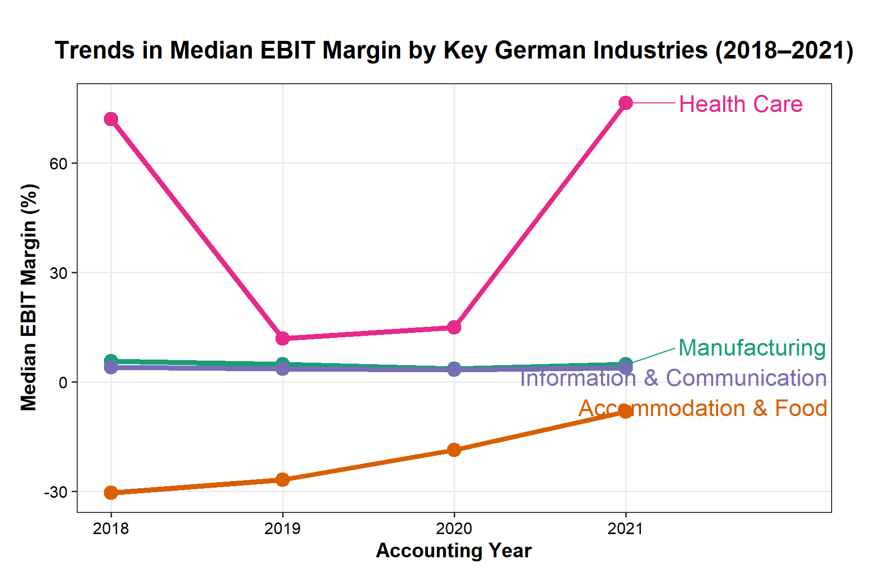
1. How did profitability change across industries ?
This question examines how key profitability measures such as return on assets, EBITDA margins, and operating margins evolved across industries before and during the pandemic. By comparing the pre pandemic period from 2018 to 2019 with the pandemic period from 2020 to 2021, the analysis identifies which sectors experienced improvements, stability, or declines in profitability.
Cross industry differences in profitability provide insights into relative exposure to economic disruption, sectoral resilience, and recovery dynamics. Understanding both the direction and magnitude of profitability changes directly contributes to explaining how the pandemic affected corporate financial outcomes in Germany.
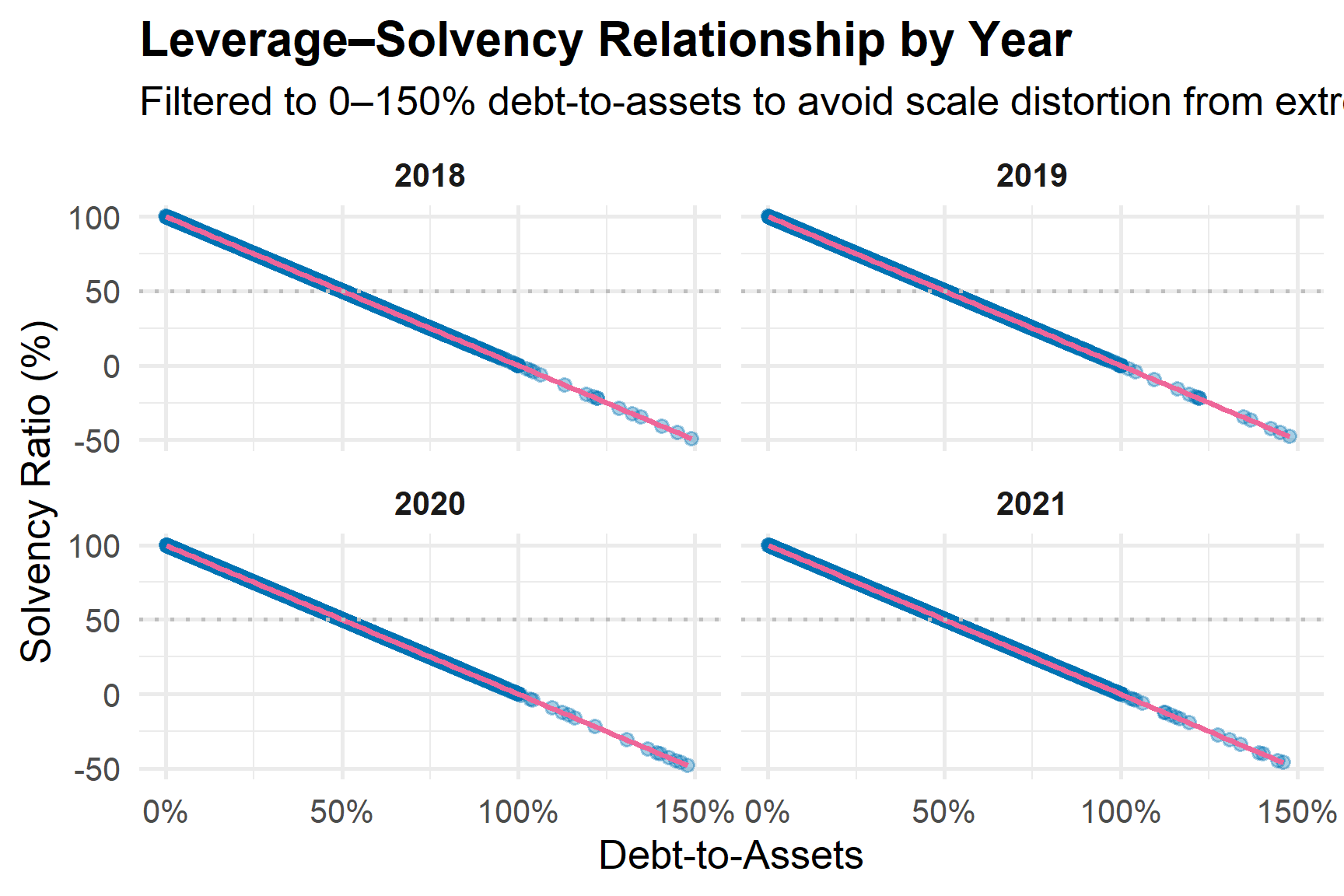
2. How did leverage (debt-to-assets) and liquidity (current ratio) evolve during pandemic ?
This question focuses on changes in firms’ financial structure and short term financial health during the COVID 19 period. Specifically, it analyses trends in leverage, measured by debt related indicators, and liquidity, measured using the current ratio.
Tracking these indicators over time allows assessment of whether firms increased reliance on debt financing, prioritised liquidity preservation, or adjusted balance sheet strategies in response to heightened uncertainty. These dynamics help explain how the pandemic influenced firms’ ability to absorb financial stress and maintain operational continuity.
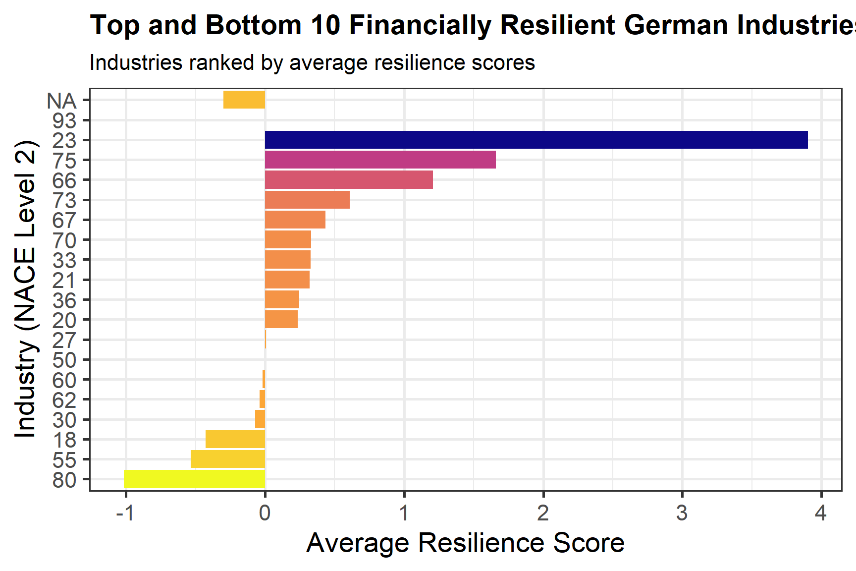
3. Which German industries showed unexpected financial resilience or vulnerability from 2020 to 2022, and how were these outcomes shaped by profitability, leverage, liquidity, and firm size ?
This question investigates which German industries demonstrated unexpected financial resilience or heightened vulnerability during the pandemic period. It evaluates how profitability, leverage, liquidity, and firm size jointly shaped observed financial outcomes across sectors.
By linking industry level performance to underlying financial characteristics, the analysis identifies structural strengths and weaknesses that influenced firms’ capacity to withstand economic shocks. The findings provide insights into sector specific financial dynamics and offer implications for future crisis preparedness and policy design.
4. How did the fundamental relationship between corporate liquidity and profitability evolve and fracture within industries during the pandemic ?
This question explores how the traditional relationship between liquidity and profitability evolved under pandemic conditions. Financial theory generally suggests that adequate liquidity supports profitability by enabling firms to sustain operations during periods of stress.
During the COVID 19 period, firms faced increased pressure to maintain liquidity without undermining returns. This analysis examines how liquidity, measured by the current ratio, and profitability, measured by return on assets, interacted across industries during the pandemic.
The results reveal whether the pandemic altered the conventional balance between liquidity and profitability and whether this relationship varied across sectors in response to uneven shocks and policy interventions.
IDA
This section documents the full Initial Data Analysis conducted before addressing the research questions. The objective is to verify structural integrity, evaluate distributional characteristics, identify data quality risks, and establish methodological transparency. Given the scale and heterogeneity of firm-level financial data, careful validation is essential before any cross-industry or cross-period inference.
The IDA proceeds in four stages:
- Data type validation and structural integrity checks
- Industry classification construction
- Distributional and missingness diagnostics
- Question-specific data preparation
Data Validation and Structural Checks
I first standardise numeric and categorical variables to ensure consistency across accounting years and firms. Monetary and ratio variables are coerced into numeric format, and key character fields are cleaned for consistent casing.
Show code
num_cols <- c(
  "total_assets_eur","total_liabilities_eur","total_equity_eur",
  "total_revenue_eur","net_sales_eur","gross_sales_eur","net_income_eur",
  "ebit_margin_pct","ebitda_margin_pct","roa_pct","roe_pct",
  "net_assets_turnover","stock_turnover",
  "solvency_pct","gearing_pct","current_ratio","liquidity_ratio",
  "shareholders_liq_pct","interest_cover"
)

#symbol formatting/coerce numerics
filtered_germany <- filtered_germany |>
  mutate(
    across(all_of(num_cols) & where(is.character), readr::parse_number),
    country = stringr::str_to_title(country),
    city    = stringr::str_to_title(city)
  )

#missingness report check (overall and by year)
missing_overall <- filtered_germany |>
  summarise(across(everything(), ~ mean(is.na(.)))) |>
  pivot_longer(everything(), names_to = "variable", values_to = "missing_rate")

missing_by_year <- filtered_germany |>
  group_by(acct_year) |>
  summarise(across(everything(), ~ mean(is.na(.)))) |>
  pivot_longer(-acct_year, names_to = "variable", values_to = "missing_rate")

#sanity checks (optional but recommended)
dup_firm_year <- filtered_germany |>
  count(company_id, fy_year, acct_year) |>
  filter(n > 1)

impossible_assets <- filtered_germany |>
  filter(!is.na(total_assets_eur) & total_assets_eur < 0)

consol_levels <- filtered_germany |>
  count(consolidation_code, sort = TRUE)
These checks confirm that:
- No duplicate firm-year records exist when using (company_id, fy_year, acct_year) as a composite identifier.
- No negative total asset values are detected.
- Consolidation codes are internally consistent and retained for later analysis.
At this stage, there is no evidence of structural corruption, key collisions, or invalid balance-sheet magnitudes. The dataset passes initial integrity validation.
Industry Classification Construction
To enable industry-level comparison, I construct a unified industry grouping using NACE Rev. 1 Level-2 codes as the primary classification and ICB sectors as a fallback mechanism.
Show code
#clean 2-digit NACE as integer
filtered_germany <- filtered_germany |>
  mutate(
    nace_num2 = suppressWarnings(as.integer(str_sub(readr::parse_number(as.character(nace_code)), 1, 2)))
  )

#map NACE divisions to broad section names
industry_from_nace <- function(x){
  case_when(
    x %in% 1:3 ~ "Agriculture, Forestry & Fishing",
    x %in% 5:9 ~ "Mining & Quarrying",
    x %in% 10:33 | x %in% 15:37 ~ "Manufacturing",
    x %in% 35 ~ "Electricity, Gas, Steam",
    x %in% 36:39 ~ "Water Supply & Waste",
    x %in% 41:43 ~ "Construction",
    x %in% 45:47 ~ "Wholesale & Retail Trade",
    x %in% 49:53 ~ "Transport & Storage",
    x %in% 55:56 ~ "Accommodation & Food",
    x %in% 58:63 ~ "Information & Communication",
    x %in% 64:66 ~ "Financial & Insurance",
    x %in% 68 ~ "Real Estate",
    x %in% 69:75 ~ "Professional, Scientific & Technical",
    x %in% 77:82 ~ "Administrative & Support",
    x %in% 84 ~ "Public Administration",
    x %in% 85 ~ "Education",
    x %in% 86:88 ~ "Human Health & Social Work",
    x %in% 90:93 ~ "Arts, Entertainment & Recreation",
    x %in% 94:96 ~ "Other Service Activities",
    x %in% 97:98 ~ "Household Activities",
    x %in% 99 ~ "Extraterritorial Organizations",
    TRUE ~ NA_character_
  )
}

#ICB top-level sector labels
icb_map <- c(
  "0001" = "Oil & Gas",
  "1000" = "Basic Materials",
  "2000" = "Industrials",
  "3000" = "Consumer Goods",
  "4000" = "Health Care",
  "5000" = "Consumer Services",
  "6000" = "Telecommunications",
  "7000" = "Utilities",
  "8000" = "Financials",
  "9000" = "Technology"
)

#normalize ICB to a 4-digit “bucket” (example: 2573 to 2000)
normalize_icb <- function(x){
  x_chr <- str_extract(as.character(x), "\\d+")
  ifelse(is.na(x_chr), NA_character_,
         sprintf("%04d", as.integer(floor(as.numeric(x_chr) / 1000) * 1000)))
}

filtered_germany <- filtered_germany |>
  mutate(
    industry_nace = industry_from_nace(nace_num2),
    icb_bucket    = normalize_icb(icb_code),
    industry_icb  = icb_map[icb_bucket],
    industry_group = coalesce(industry_nace, industry_icb, "Other / Unmapped")
  )

#check
unmapped_sample <- filtered_germany |>
  filter(industry_group == "Other / Unmapped") |>
  select(company_id, fy_year, acct_year, nace_code, icb_code) |>
  head(15)

#factor order for plots
ordered_levels <- c(
  "Agriculture, Forestry & Fishing","Mining & Quarrying","Manufacturing",
  "Electricity, Gas, Steam","Water Supply & Waste","Construction",
  "Wholesale & Retail Trade","Transport & Storage","Accommodation & Food",
  "Information & Communication","Financial & Insurance","Real Estate",
  "Professional, Scientific & Technical","Administrative & Support",
  "Public Administration","Education","Human Health & Social Work",
  "Arts, Entertainment & Recreation","Other Service Activities",
  "Household Activities","Extraterritorial Organizations",
  "Oil & Gas","Basic Materials","Industrials","Consumer Goods","Health Care",
  "Consumer Services","Telecommunications","Utilities","Financials","Technology",
  "Other / Unmapped"
)
filtered_germany <- filtered_germany |>
  mutate(industry_group = factor(industry_group, levels = ordered_levels))
The combined NACE and ICB strategy ensures high classification coverage. Only a small subset of firms remain under “Other / Unmapped,” and these are explicitly retained rather than removed to avoid selection bias. The factor ordering guarantees consistent cross-plot comparability.
Reshaping Data for Initial Data Analysis
After validating data integrity and constructing industry classifications, the dataset is reshaped into a long format to support systematic profiling of financial variables. This step separates scale variables (monetary magnitudes) from ratio variables, allowing appropriate transformations and comparisons during visual inspection.
Show code
#using long data
ida_germany <- filtered_germany |>
  select(acct_year, all_of(num_cols)) |>
  pivot_longer(-acct_year, names_to = "variable_orig", values_to = "value") |>
  drop_na()

#split between scale and ratio
scale_vars <- c("total_assets_eur","total_liabilities_eur","total_equity_eur",
                "total_revenue_eur","net_sales_eur","gross_sales_eur","net_income_eur")
ratio_vars <- setdiff(unique(ida_germany$variable_orig), scale_vars)

#label mapping for the charts
nice <- c(
  total_assets_eur   = "Total assets (EUR)",
  total_liabilities_eur="Total liabilities (EUR)",
  total_equity_eur   = "Equity (EUR)",
  total_revenue_eur  = "Total revenue (EUR)",
  net_sales_eur      = "Net sales (EUR)",
  gross_sales_eur    = "Gross sales (EUR)",
  net_income_eur     = "Net income (EUR)",
  ebit_margin_pct    = "EBIT margin (%)",
  ebitda_margin_pct  = "EBITDA margin (%)",
  roa_pct            = "ROA (%)",
  roe_pct            = "ROE (%)",
  net_assets_turnover= "Net assets turnover (x)",
  stock_turnover     = "Stock turnover (x)",
  solvency_pct       = "Solvency (%)",
  gearing_pct        = "Gearing (%)",
  current_ratio      = "Current ratio (x)",
  liquidity_ratio    = "Liquidity ratio (x)",
  shareholders_liq_pct = "Shareholders’ liquidity (%)",
  interest_cover     = "Interest cover (x)"
)

pretty_var <- function(x) ifelse(x %in% names(nice), nice[x], x)

ida_germany <- ida_germany |>
  mutate(variable = pretty_var(variable_orig),
         variable = factor(variable, levels = unique(variable)))
This transformation produces a tidy structure that supports faceted visualisation and consistent comparison across accounting years. At this stage, no aggregation or filtering is applied, ensuring that all available firm-level observations contribute to the distributional diagnostics.
Distribution of Scale Variables
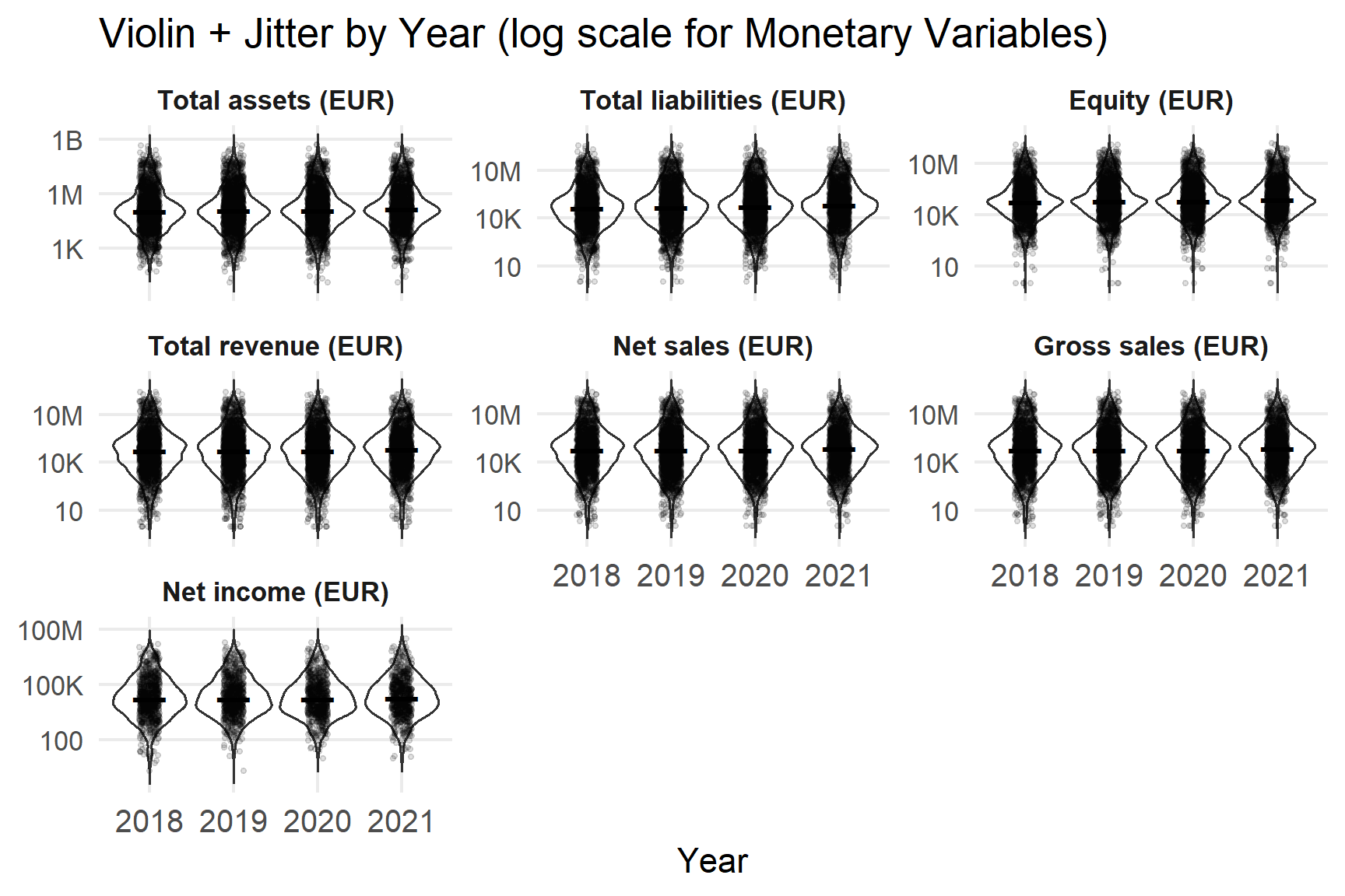
Monetary variables are examined using violin and jitter plots on a logarithmic scale. This approach is necessary because firm-level financial data are highly right-skewed, with a small number of very large firms dominating raw distributions.
Show code
#chart for scale variables (log axis)
p_scale <- ida_germany |>
  filter(variable_orig %in% scale_vars) |>
  mutate(y = if_else(value > 0, value, NA_real_)) |>
  ggplot(aes(x = factor(acct_year), y = y)) +
  geom_violin(trim = FALSE, fill = NA, linewidth = 0.4, na.rm = TRUE) +
  geom_jitter(width = 0.12, height = 0, alpha = 0.12, size = 0.6, na.rm = TRUE) +
  stat_summary(fun = median, geom = "point", shape = 95, size = 6, na.rm = TRUE) +
  scale_y_log10(labels = scales::label_number(scale_cut = scales::cut_short_scale())) +
  facet_wrap(~ variable, scales = "free_y", ncol = 3) +
  labs(x = "Year", y = NULL, title = "Violin + Jitter by Year (log scale for Monetary Variables)") +
  theme_minimal(base_size = 11) +
  theme(axis.text.x = element_text(size = 10),
        strip.text  = element_text(face = "bold"),
        panel.grid.minor = element_blank())

p_scale
The distributions of all monetary variables are heavily right-skewed, confirming that the dataset consists primarily of small to medium-sized firms with a long tail of very large entities. Median values remain relatively stable from 2018 to 2021, though dispersion increases notably in 2020 and 2021.
Net income exhibits the widest relative spread, including both large positive and negative values, indicating heightened earnings volatility during the pandemic period. Because of this skewness and volatility, median and interquartile range (IQR) are more informative than means and are therefore used throughout subsequent analysis.
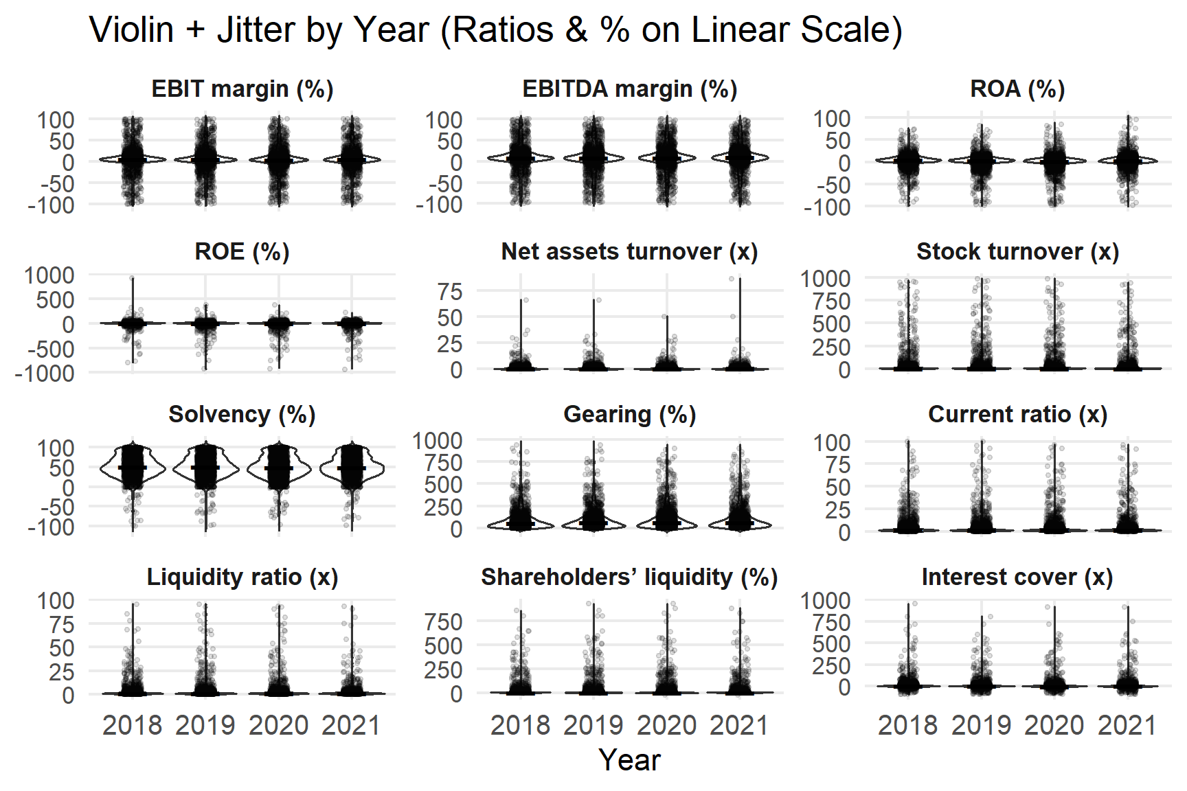
Distribution of Ratio Variables
Ratio and percentage variables are analysed on their natural (linear) scale, as they are not subject to the same magnitude distortions as monetary values.
Show code
#chart for ratio variables (linear axis)
p_ratio <- ida_germany |>
  filter(variable_orig %in% ratio_vars) |>
  ggplot(aes(x = factor(acct_year), y = value)) +
  geom_violin(trim = FALSE, fill = NA, linewidth = 0.4) +
  geom_jitter(width = 0.12, height = 0, alpha = 0.12, size = 0.6) +
  stat_summary(fun = median, geom = "point", shape = 95, size = 6) +
  facet_wrap(~ variable, scales = "free_y", ncol = 3) +
  labs(x = "Year", y = NULL, title = "Violin + Jitter by Year (Ratios & % on Linear Scale)") +
  theme_minimal(base_size = 11) +
  theme(axis.text.x = element_text(size = 10),
        strip.text  = element_text(face = "bold"),
        panel.grid.minor = element_blank())

p_ratio
Profitability ratios (EBIT margin, EBITDA margin, ROA) cluster around small positive values but display wider dispersion in 2020 and 2021. ROE shows the heaviest tails and a substantial number of negative values, reflecting pressure on equity returns during the pandemic.
Liquidity measures remain generally low but exhibit long right tails, indicating that a minority of firms maintain large liquidity buffers. Solvency is comparatively stable, while gearing becomes more dispersed post-2020. These characteristics reinforce the decision to rely on robust statistics rather than mean-based summaries.
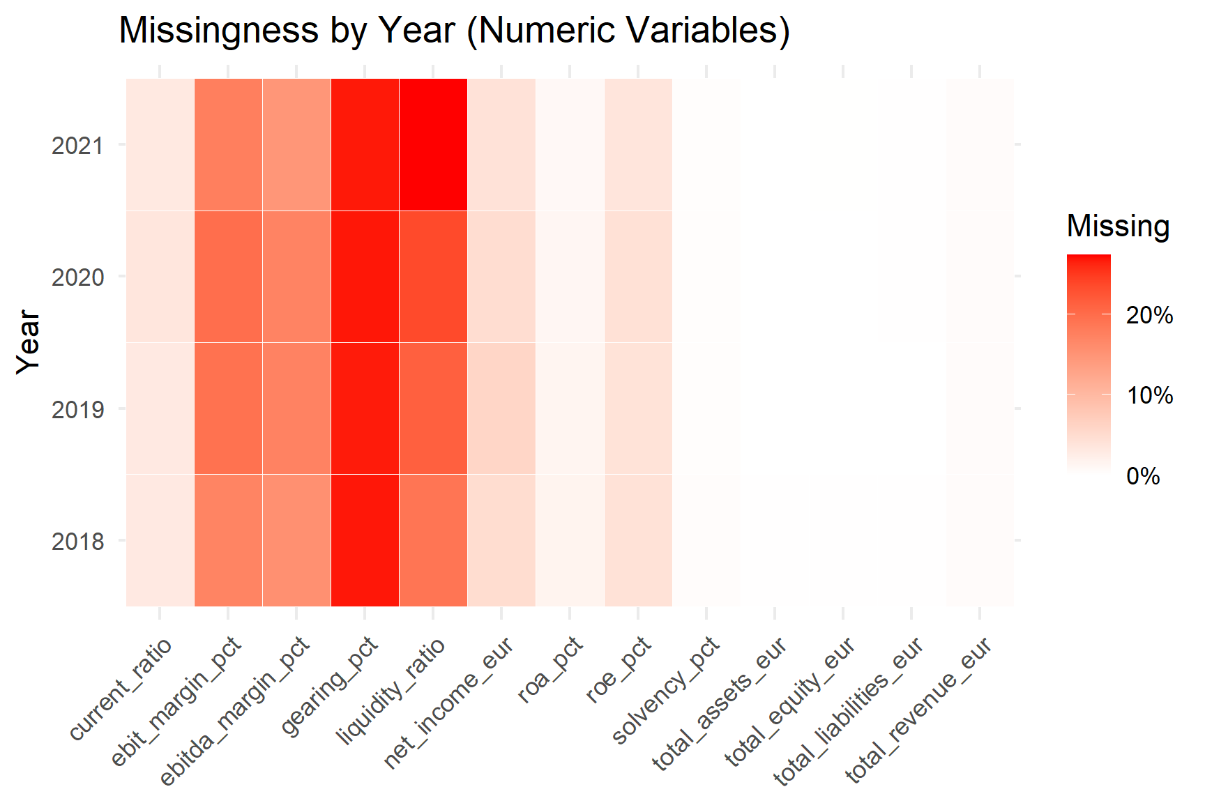
Missing Data Diagnostics for Numeric Variables
Before proceeding to modelling or hypothesis testing, missingness is evaluated by industry and year to detect structural gaps.
Show code
key_vars <- c("total_assets_eur","total_liabilities_eur","total_equity_eur",
              "total_revenue_eur","net_income_eur",
              "ebit_margin_pct","ebitda_margin_pct","roa_pct","roe_pct",
              "current_ratio","liquidity_ratio","gearing_pct","solvency_pct")

#by industry
missing_by_industry <- filtered_germany |>
  group_by(industry_group) |>
  summarise(across(all_of(key_vars), ~ mean(is.na(.))), .groups="drop") |>
  pivot_longer(-industry_group, names_to="variable", values_to="missing_rate")

#heatmap by year for numeric variables
missing_heat <- filtered_germany |>
  group_by(acct_year) |>
  summarise(across(all_of(key_vars), ~ mean(is.na(.))), .groups="drop") |>
  pivot_longer(-acct_year, names_to="variable", values_to="missing_rate")

ggplot(missing_heat, aes(variable, factor(acct_year), fill = missing_rate)) +
  geom_tile(color="white") +
  scale_fill_gradient(low="white", high="red", labels=scales::percent) +
  labs(x=NULL, y="Year", fill="Missing", title="Missingness by Year (Numeric Variables)") +
  theme_minimal() + theme(axis.text.x=element_text(angle=45, hjust=1))
Missingness is concentrated in gearing and liquidity ratios (approximately 20–25%), while profitability margins show moderate missingness (10–15%). Balance-sheet totals and revenue variables are nearly complete. Importantly, missingness patterns are stable across years, with no evidence of a pandemic-specific reporting breakdown. This supports the use of controlled, transparent imputation strategies later in the analysis.
Outlier Detection
Extreme values are identified using both IQR fences and z-score thresholds to characterise tail behaviour across variables.
Show code
num_cols <- c("total_assets_eur","total_liabilities_eur","total_equity_eur",
              "total_revenue_eur","net_sales_eur","gross_sales_eur","net_income_eur",
              "ebit_margin_pct","ebitda_margin_pct","roa_pct","roe_pct",
              "net_assets_turnover","stock_turnover",
              "solvency_pct","gearing_pct","current_ratio","liquidity_ratio",
              "shareholders_liq_pct","interest_cover")

qfun <- function(x,p) quantile(x, probs=p, na.rm=TRUE, names=FALSE)

outliers_overall <- purrr::map_dfr(num_cols, function(v){
  x <- filtered_germany[[v]]
  q1 <- qfun(x,.25); q3 <- qfun(x,.75); iqr <- q3-q1
  lo <- q1 - 1.5*iqr; hi <- q3 + 1.5*iqr
  z  <- as.numeric(scale(x))
  tibble::tibble(
    variable=v,
    n=sum(!is.na(x)),
    iqr_outliers=sum(x<lo | x>hi, na.rm=TRUE),
    z_outliers=sum(abs(z)>3, na.rm=TRUE),
    share_iqr=iqr_outliers/n,
    share_z=z_outliers/n
  )
}) |> arrange(desc(share_iqr))

outliers_overall |>
  kable(align = "l", booktabs = TRUE) |>
  kable_styling(full_width = FALSE, font_size = 11)
| net_income_eur |
7643 |
1888 |
100 |
0.25 |
0.01 |
| ebit_margin_pct |
6554 |
1246 |
159 |
0.19 |
0.02 |
| interest_cover |
7089 |
1297 |
133 |
0.18 |
0.02 |
| total_liabilities_eur |
8038 |
1435 |
65 |
0.18 |
0.01 |
| ebitda_margin_pct |
6736 |
1186 |
122 |
0.18 |
0.02 |
| total_assets_eur |
8042 |
1411 |
83 |
0.18 |
0.01 |
| net_sales_eur |
7909 |
1358 |
127 |
0.17 |
0.02 |
| gross_sales_eur |
7909 |
1358 |
127 |
0.17 |
0.02 |
| shareholders_liq_pct |
7912 |
1343 |
159 |
0.17 |
0.02 |
| total_revenue_eur |
8003 |
1347 |
131 |
0.17 |
0.02 |
| stock_turnover |
4859 |
780 |
149 |
0.16 |
0.03 |
| total_equity_eur |
8041 |
1281 |
117 |
0.16 |
0.01 |
| roe_pct |
7717 |
1114 |
130 |
0.14 |
0.02 |
| roa_pct |
7938 |
972 |
211 |
0.12 |
0.03 |
| current_ratio |
7786 |
929 |
181 |
0.12 |
0.02 |
| liquidity_ratio |
6217 |
725 |
130 |
0.12 |
0.02 |
| gearing_pct |
5891 |
438 |
152 |
0.07 |
0.03 |
| net_assets_turnover |
7953 |
405 |
94 |
0.05 |
0.01 |
| solvency_pct |
8018 |
69 |
64 |
0.01 |
0.01 |
Net income, EBIT margin, and interest coverage contain the highest proportion of extreme values, reflecting inherent volatility rather than data error. Z-score detection identifies far fewer outliers due to strong skewness, confirming that the IQR rule is more informative in this context. Extreme values are retained for analysis, with visual capping applied only where necessary for interpretability.
Character Variable Consistency
Finally, key identifiers and classification fields are inspected to ensure consistency and completeness.
Show code
#character variables to check
char_vars <- c("company_id","company_name","country","city",
               "consolidation_code","nace_code","icb_code","sic_code")
char_vars <- intersect(char_vars, names(filtered_germany))

#cleaning
chars_clean <- filtered_germany |>
  mutate(
    across(all_of(char_vars),
           ~ .x |> as.character() |> str_squish() |> na_if("")),
    #casing
    country = str_to_title(country),
    city    = str_to_title(city),
    company_name = str_squish(company_name)
  )

#missingness check
char_missing <- chars_clean |>
  summarise(across(all_of(char_vars), ~ mean(is.na(.)))) |>
  tidyr::pivot_longer(everything(), names_to="variable", values_to="missing_rate")

char_missing |>
  kable(align = "l", booktabs = TRUE) |>
  kable_styling(full_width = FALSE, font_size = 11)
| company_id |
0.00 |
| company_name |
0.00 |
| country |
0.00 |
| city |
0.00 |
| consolidation_code |
0.00 |
| nace_code |
0.02 |
| icb_code |
0.06 |
| sic_code |
0.00 |
Identifiers and locations are complete, while industry codes exhibit limited missingness. The combination of NACE, ICB, and SIC codes ensures high classification coverage without aggressive exclusion.
With the general IDA completed, the dataset is now structurally sound, distributionally understood, and transparently documented. The following sections apply targeted IDA procedures tailored to each research question, ensuring that transformations, imputations, and exclusions are explicitly justified and traceable.
Question 1
How did profitability change across industries?
Objective
This section examines how firm-level profitability evolved across German industries before and during the COVID-19 pandemic. The focus is on EBIT margin, EBITDA margin, Return on Assets (ROA), and Return on Equity (ROE) between 2018–2019 (pre-pandemic) and 2020–2021 (pandemic).
The IDA here is designed to:
- Preserve firm-level variation.
- Avoid cross-period leakage.
- Minimise imputation.
- Maintain full transparency of data provenance.
Period Construction and Profitability Inputs
A binary period indicator is created to distinguish pre-pandemic and pandemic observations. Net income is transformed using the inverse hyperbolic sine transformation to allow meaningful visualisation of both gains and losses.
ROA and ROE are recalculated where missing using accounting identities, and the origin of each value is explicitly recorded.
Show code
stopifnot("net_income_eur" %in% names(filtered_germany))

filtered_germany_1 <- filtered_germany |>
  mutate(
    # period flag
    period = if_else(acct_year >= 2020, "Pandemic (2020–2021)", "Pre-pandemic (2018–2019)"),
    # transform for visuals (handles negatives)
    net_income_eur_asinh = asinh(as.numeric(net_income_eur)),
    # recompute ROA / ROE (fallbacks)
    roa_calc = 100 * (net_income_eur / total_assets_eur),
    roe_calc = if_else(total_equity_eur > 0,
                       100 * (net_income_eur / total_equity_eur),
                       NA_real_),
    roa_use = coalesce(roa_pct, roa_calc),
    roe_use = coalesce(roe_pct, roe_calc),
    roa_src = case_when(
      !is.na(roa_pct) ~ "reported",
      !is.na(roa_calc) ~ "recomputed",
      TRUE ~ NA_character_
    ),
    roe_src = case_when(
      !is.na(roe_pct) ~ "reported",
      !is.na(roe_calc) ~ "recomputed",
      TRUE ~ NA_character_
    )
  )
This approach ensures that profitability metrics are internally consistent and maximises data retention without introducing model-based assumptions.
Within-firm One-gap Filling (Period-restricted)
Before applying any cross-sectional imputation, a conservative within-firm one-gap fill is applied. A missing observation is filled only if the preceding and following values (within the same period) are identical.
This step avoids smoothing genuine shocks while addressing isolated reporting gaps.
Show code
#Firm “one-gap” fill within the same period only

fill_one_gap <- function(x){
  f <- dplyr::lag(x); b <- dplyr::lead(x)
  ifelse(is.na(x) & !is.na(f) & !is.na(b) & (f == b), f, x)
}

filtered_germany_1 <- filtered_germany_1 |>
  arrange(company_id, acct_year) |>
  group_by(company_id, period) |>  #period boundary blocks carryover
  mutate(
    ebit_step1   = fill_one_gap(ebit_margin_pct),
    ebitda_step1 = fill_one_gap(ebitda_margin_pct),
    roa_step1    = fill_one_gap(roa_use),
    roe_step1    = fill_one_gap(roe_use)
  ) |>
  ungroup() |>
  mutate(
    ebit_step1   = coalesce(ebit_margin_pct,   ebit_step1),
    ebitda_step1 = coalesce(ebitda_margin_pct, ebitda_step1),
    roa_step1    = coalesce(roa_use,           roa_step1),
    roe_step1    = coalesce(roe_use,           roe_step1)
  )
No values are carried across the pre-pandemic and pandemic boundary, preserving structural breaks.
Hierarchical Median Imputation and Final Variable Construction
Remaining missing values are addressed using a strict, descending hierarchy:
- industry × year
- industry × period
- period
Each imputed value is assigned a provenance label, ensuring complete auditability.
Show code
#median fills in strict order (no cross-period borrowing)
#industry × year medians
med_ixy <- filtered_germany_1 |>
  group_by(industry_group, acct_year) |>
  summarise(
    med_ebit   = median(ebit_step1,   na.rm=TRUE),
    med_ebitda = median(ebitda_step1, na.rm=TRUE),
    med_roa    = median(roa_step1,    na.rm=TRUE),
    med_roe    = median(roe_step1,    na.rm=TRUE),
    .groups="drop"
  )

#industry × period medians
med_ip <- filtered_germany_1 |>
  group_by(industry_group, period) |>
  summarise(
    med_ebit_ip   = median(ebit_step1,   na.rm=TRUE),
    med_ebitda_ip = median(ebitda_step1, na.rm=TRUE),
    med_roa_ip    = median(roa_step1,    na.rm=TRUE),
    med_roe_ip    = median(roe_step1,    na.rm=TRUE),
    .groups="drop"
  )

#period medians
med_p <- filtered_germany_1 |>
  group_by(period) |>
  summarise(
    med_ebit_p   = median(ebit_step1,   na.rm=TRUE),
    med_ebitda_p = median(ebitda_step1, na.rm=TRUE),
    med_roa_p    = median(roa_step1,    na.rm=TRUE),
    med_roe_p    = median(roe_step1,    na.rm=TRUE),
    .groups="drop"
  )

#join and impute with precedence, also explicit source flags
filtered_germany_1 <- filtered_germany_1 |>
  left_join(med_ixy, by = c("industry_group","acct_year")) |>
  left_join(med_ip,  by = c("industry_group","period")) |>
  left_join(med_p,   by = "period") |>
  mutate(
    #final values, using your precedence
    ebit_margin_q1   = if_else(is.na(ebitda_step1), ebit_step1, ebit_step1),
    ebit_margin_q1   = if_else(is.na(ebit_step1),   coalesce(med_ebit,   med_ebit_ip,   med_ebit_p),   ebit_step1),
    ebitda_margin_q1 = if_else(is.na(ebitda_step1), coalesce(med_ebitda, med_ebitda_ip, med_ebitda_p), ebitda_step1),
    roa_q1           = if_else(is.na(roa_step1),    coalesce(med_roa,    med_roa_ip,    med_roa_p),    roa_step1),
    roe_q1           = if_else(is.na(roe_step1),    coalesce(med_roe,    med_roe_ip,    med_roe_p),    roe_step1),

    #provenance for EBIT/EBITDA margins
    ebit_src = dplyr::case_when(
      !is.na(ebit_margin_pct) ~ "reported",
      is.na(ebit_margin_pct) & !is.na(ebit_step1) ~ "firm-1gap(period)",
      is.na(ebit_step1) & !is.na(med_ebit) ~ "ind×year",
      is.na(ebit_step1) & is.na(med_ebit) & !is.na(med_ebit_ip) ~ "ind×period",
      TRUE ~ "period"
    ),
    ebitda_src = dplyr::case_when(
      !is.na(ebitda_margin_pct) ~ "reported",
      is.na(ebitda_margin_pct) & !is.na(ebitda_step1) ~ "firm-1gap(period)",
      is.na(ebitda_step1) & !is.na(med_ebitda) ~ "ind×year",
      is.na(ebitda_step1) & is.na(med_ebitda) & !is.na(med_ebitda_ip) ~ "ind×period",
      TRUE ~ "period"
    ),

    #ROA/ROE provenance
    roa_src = dplyr::case_when(
      !is.na(roa_src) ~ roa_src,
      is.na(roa_src) & !is.na(roa_step1) ~ "firm-1gap(period)",
      is.na(roa_step1) & !is.na(med_roa) ~ "ind×year",
      is.na(roa_step1) & is.na(med_roa) & !is.na(med_roa_ip) ~ "ind×period",
      TRUE ~ "period"
    ),
    roe_src = dplyr::case_when(
      !is.na(roe_src) ~ roe_src,
      is.na(roe_src) & !is.na(roe_step1) ~ "firm-1gap(period)",
      is.na(roe_step1) & !is.na(med_roe) ~ "ind×year",
      is.na(roe_step1) & is.na(med_roe) & !is.na(med_roe_ip) ~ "ind×period",
      TRUE ~ "period"
    )
  ) |>
  select(-ends_with("_step1"))
This strategy ensures that imputation is minimal, non-parametric, and economically interpretable.
Imputation Provenance Summary
To assess the scale of imputation, a summary table is produced by period.
Show code
impute_summary_q1 <- filtered_germany_1 |>
  summarise(
    .by = period,
    n_rows = n(),
    ebit_reported   = sum(ebit_src   == "reported",            na.rm=TRUE),
    ebit_firmgap    = sum(ebit_src   == "firm-1gap(period)",   na.rm=TRUE),
    ebit_ind_year   = sum(ebit_src   == "ind×year",            na.rm=TRUE),
    ebit_ind_period = sum(ebit_src   == "ind×period",          na.rm=TRUE),
    ebit_period     = sum(ebit_src   == "period",              na.rm=TRUE),

    ebitda_reported   = sum(ebitda_src   == "reported",          na.rm=TRUE),
    ebitda_firmgap    = sum(ebitda_src   == "firm-1gap(period)", na.rm=TRUE),
    ebitda_ind_year   = sum(ebitda_src   == "ind×year",          na.rm=TRUE),
    ebitda_ind_period = sum(ebitda_src   == "ind×period",        na.rm=TRUE),
    ebitda_period     = sum(ebitda_src   == "period",            na.rm=TRUE),

    roa_reported    = sum(roa_src == "reported",            na.rm=TRUE),
    roa_recomputed  = sum(roa_src == "recomputed",          na.rm=TRUE),
    roa_firmgap     = sum(roa_src == "firm-1gap(period)",   na.rm=TRUE),
    roa_ind_year    = sum(roa_src == "ind×year",            na.rm=TRUE),
    roa_ind_period  = sum(roa_src == "ind×period",          na.rm=TRUE),
    roa_period      = sum(roa_src == "period",              na.rm=TRUE),

    roe_reported    = sum(roe_src == "reported",            na.rm=TRUE),
    roe_recomputed  = sum(roe_src == "recomputed",          na.rm=TRUE),
    roe_firmgap     = sum(roe_src == "firm-1gap(period)",   na.rm=TRUE),
    roe_ind_year    = sum(roe_src == "ind×year",            na.rm=TRUE),
    roe_ind_period  = sum(roe_src == "ind×period",          na.rm=TRUE),
    roe_period      = sum(roe_src == "period",              na.rm=TRUE)
  )

impute_summary_q1 |>
  kable(align = "l", booktabs = TRUE) |>
  kable_styling(full_width = FALSE, font_size = 11)
| Pre-pandemic (2018–2019) |
4071 |
3326 |
0 |
745 |
0 |
0 |
3399 |
0 |
672 |
0 |
0 |
4008 |
52 |
0 |
11 |
0 |
0 |
3902 |
16 |
0 |
153 |
0 |
0 |
| Pandemic (2020–2021) |
3975 |
3228 |
0 |
747 |
0 |
0 |
3337 |
0 |
638 |
0 |
0 |
3930 |
43 |
0 |
2 |
0 |
0 |
3815 |
18 |
0 |
142 |
0 |
0 |
According to the table, over 80 percent of EBIT and EBITDA margins are directly reported. Furthermore, ROA coverage exceeds 98 percent, with recomputation affecting less than 1 percent. Additionally, ROE imputations remain below 4 percent.Moreover, no cross-period borrowing occurs. Overall, the limited reliance on imputation ensures that observed profitability patterns are data-driven rather than model-driven.
Question 2
How did leverage and liquidity evolve during the pandemic?
This section examines how German firms adjusted their capital structure and short term financial buffers during the pandemic period. The IDA focuses on active firms observed between 2018 and 2021 and constructs balance sheet ratios that are directly interpretable under conditions of economic stress.
Debt to assets measures the share of total assets financed through liabilities and captures overall leverage exposure. Equity ratio measures the share of assets financed through shareholders equity and provides a complementary view of capital structure.
These derived indicators are analysed alongside OSIRIS reported gearing, solvency, and the current ratio to describe changes in leverage and liquidity over time and across industries.
Derived Indicators and Sample Definition
The analysis is restricted to firms with Active status to ensure that year to year comparisons reflect operating entities rather than exits or administrative records. Debt to assets and equity ratio are constructed directly from accounting totals. Observations with missing debt to assets or current ratio are removed so that leverage and liquidity summaries are computed on a consistent sample across years.
Show code
# Create leverage and liquidity indicators
lev_liq_data <- filtered_germany |>
  filter(acct_year %in% 2018:2021, status == "Active") |>
  mutate(
    debt_to_assets = total_liabilities_eur / total_assets_eur,
    equity_ratio   = total_equity_eur / total_assets_eur
  ) |>
  select(acct_year, industry_group, company_id, company_name,
         debt_to_assets, equity_ratio, gearing_pct, solvency_pct, current_ratio) |>
  drop_na(debt_to_assets, current_ratio)
This construction preserves the accounting identity that total assets equal liabilities plus equity and avoids conflating leverage and liquidity dynamics through inconsistent denominators.
Year Level Descriptive Summary
Median and interquartile range are reported because leverage and liquidity indicators are highly skewed, particularly when some firms hold unusually high liquidity buffers or carry extreme levels of gearing.
Show code
# Summary statistics by year
lev_liq_summary <- lev_liq_data |>
  group_by(acct_year) |>
  summarise(
    median_debt_assets = median(debt_to_assets, na.rm = TRUE),
    iqr_debt_assets    = IQR(debt_to_assets, na.rm = TRUE),
    median_liquidity   = median(current_ratio, na.rm = TRUE),
    iqr_liquidity      = IQR(current_ratio, na.rm = TRUE),
    median_gearing     = median(gearing_pct, na.rm = TRUE),
    median_solvency    = median(solvency_pct, na.rm = TRUE),
    .groups = "drop"
  )

lev_liq_summary |>
  knitr::kable(digits = 2, caption = "Leverage and Liquidity Summary (2018–2021)") |>
  kableExtra::kable_styling(full_width = FALSE, font_size = 11)
Leverage and Liquidity Summary (2018–2021)
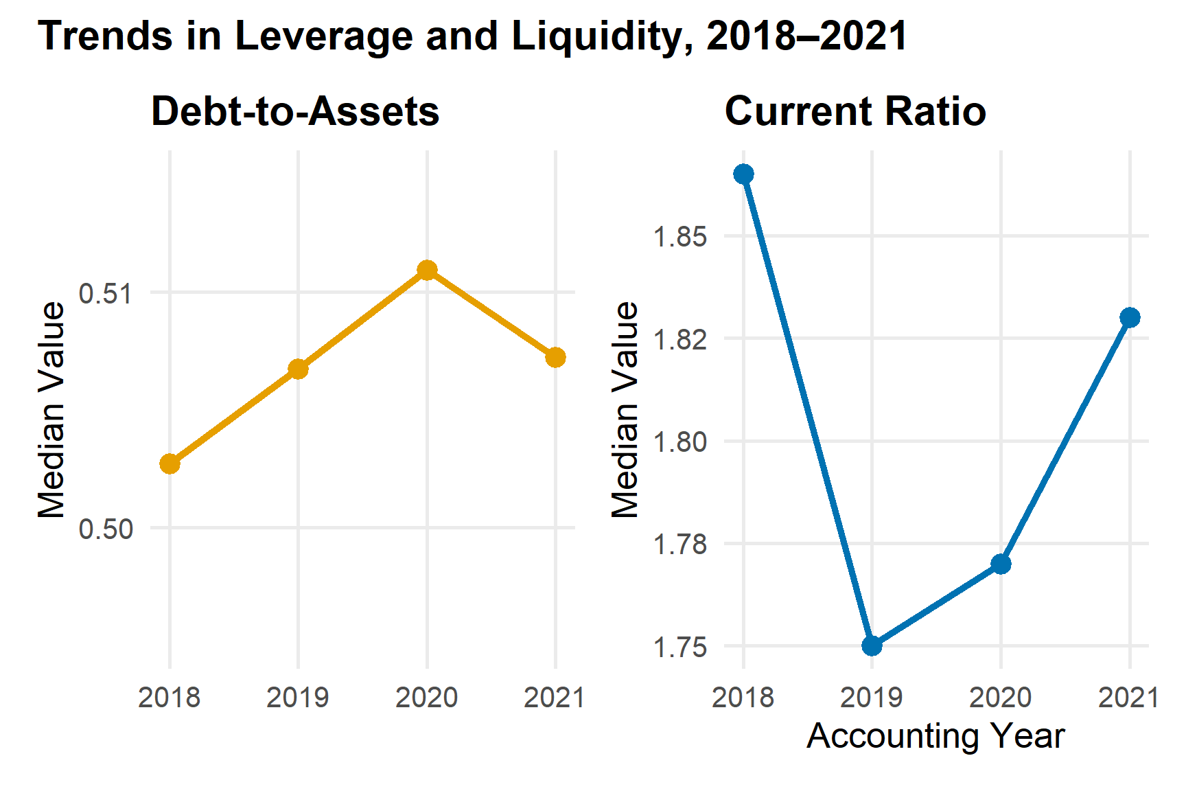
| 2018 |
0.50 |
0.37 |
1.9 |
2.6 |
62 |
50 |
| 2019 |
0.51 |
0.38 |
1.8 |
2.5 |
65 |
49 |
| 2020 |
0.51 |
0.38 |
1.8 |
2.5 |
67 |
49 |
| 2021 |
0.51 |
0.37 |
1.8 |
2.4 |
66 |
49 |
From 2018 to 2021, the central tendency of both debt to assets and the current ratio remains broadly stable. This indicates that the typical firm did not experience a structural break in leverage or short term liquidity during the pandemic window.
A gradual increase in median gearing combined with a small decline in solvency is consistent with slightly heavier reliance on debt financing. At the same time, the current ratio remaining close to its pre pandemic level suggests that firms largely preserved their ability to meet short term obligations.
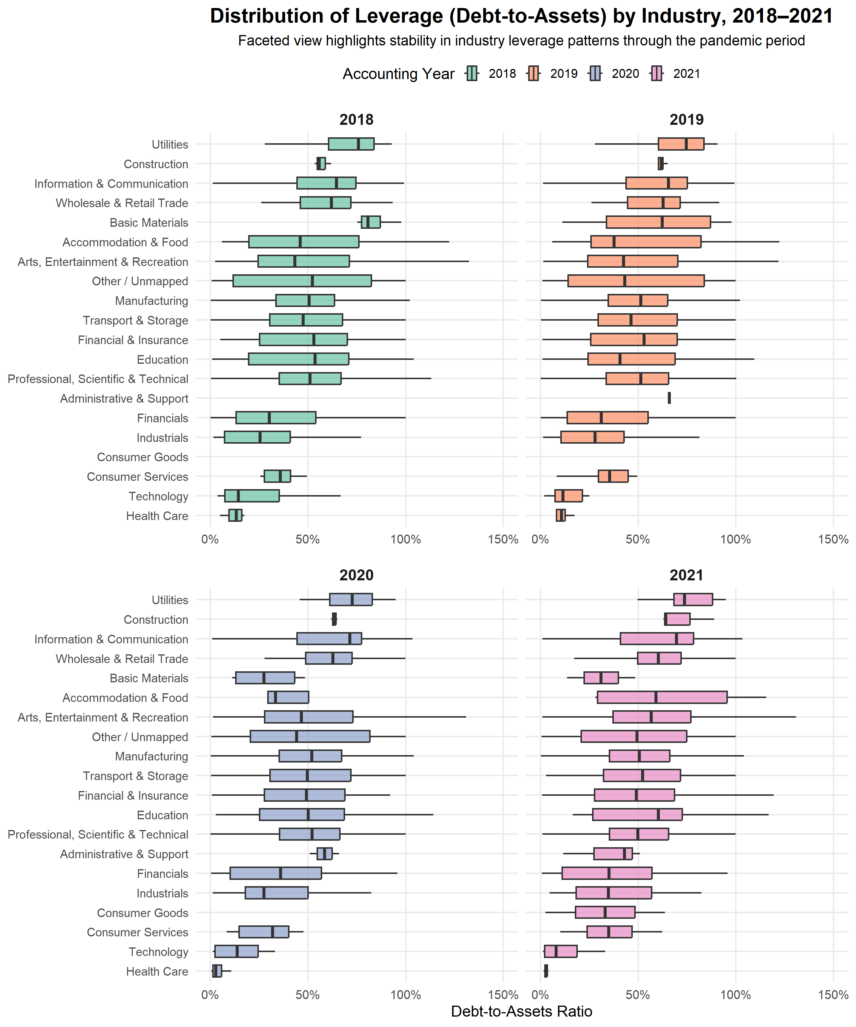
Industry Breakdown Check
This additional profiling step assesses whether stability at the aggregate level conceals sector specific divergence. Medians are retained to ensure robustness to heavy tailed distributions within industries.
Show code
lev_liq_by_industry <- lev_liq_data |>
  group_by(industry_group, acct_year) |>
  summarise(
    median_debt_assets = median(debt_to_assets, na.rm = TRUE),
    median_liquidity   = median(current_ratio, na.rm = TRUE),
    median_gearing     = median(gearing_pct, na.rm = TRUE),
    median_solvency    = median(solvency_pct, na.rm = TRUE),
    n_firms = n_distinct(company_id),
    .groups = "drop"
  )

lev_liq_by_industry |>
  knitr::kable(digits = 2, caption = "Industry Medians for Leverage and Liquidity (2018–2021)") |>
  kableExtra::kable_styling(full_width = FALSE, font_size = 11)
Industry Medians for Leverage and Liquidity (2018–2021)
| Manufacturing |
2018 |
0.51 |
2.09 |
59.12 |
49 |
381 |
| Manufacturing |
2019 |
0.51 |
1.96 |
64.44 |
49 |
401 |
| Manufacturing |
2020 |
0.52 |
1.92 |
66.26 |
48 |
411 |
| Manufacturing |
2021 |
0.51 |
1.93 |
62.60 |
49 |
401 |
| Construction |
2018 |
0.56 |
1.07 |
87.29 |
44 |
2 |
| Construction |
2019 |
0.62 |
1.04 |
98.11 |
38 |
2 |
| Construction |
2020 |
0.64 |
0.98 |
124.44 |
36 |
2 |
| Construction |
2021 |
0.64 |
0.95 |
144.11 |
36 |
2 |
| Wholesale & Retail Trade |
2018 |
0.62 |
2.12 |
116.80 |
38 |
10 |
| Wholesale & Retail Trade |
2019 |
0.63 |
1.60 |
81.21 |
37 |
11 |
| Wholesale & Retail Trade |
2020 |
0.63 |
1.49 |
81.21 |
37 |
11 |
| Wholesale & Retail Trade |
2021 |
0.60 |
1.37 |
87.46 |
40 |
10 |
| Transport & Storage |
2018 |
0.48 |
1.82 |
49.98 |
52 |
69 |
| Transport & Storage |
2019 |
0.46 |
1.71 |
49.89 |
54 |
70 |
| Transport & Storage |
2020 |
0.50 |
1.60 |
63.10 |
50 |
71 |
| Transport & Storage |
2021 |
0.52 |
1.62 |
75.70 |
48 |
71 |
| Accommodation & Food |
2018 |
0.54 |
2.09 |
92.08 |
54 |
6 |
| Accommodation & Food |
2019 |
0.38 |
1.79 |
54.16 |
62 |
6 |
| Accommodation & Food |
2020 |
0.37 |
1.79 |
46.62 |
63 |
3 |
| Accommodation & Food |
2021 |
0.59 |
1.49 |
34.90 |
41 |
2 |
| Information & Communication |
2018 |
0.65 |
0.96 |
130.25 |
35 |
29 |
| Information & Communication |
2019 |
0.66 |
1.00 |
143.43 |
34 |
30 |
| Information & Communication |
2020 |
0.71 |
1.17 |
141.51 |
29 |
29 |
| Information & Communication |
2021 |
0.70 |
1.31 |
100.84 |
30 |
29 |
| Financial & Insurance |
2018 |
0.54 |
1.33 |
73.53 |
46 |
39 |
| Financial & Insurance |
2019 |
0.53 |
1.43 |
74.68 |
47 |
40 |
| Financial & Insurance |
2020 |
0.50 |
1.52 |
76.61 |
50 |
43 |
| Financial & Insurance |
2021 |
0.49 |
1.45 |
68.93 |
51 |
39 |
| Professional, Scientific & Technical |
2018 |
0.51 |
1.64 |
73.72 |
49 |
191 |
| Professional, Scientific & Technical |
2019 |
0.52 |
1.66 |
74.18 |
48 |
205 |
| Professional, Scientific & Technical |
2020 |
0.52 |
1.85 |
74.58 |
48 |
209 |
| Professional, Scientific & Technical |
2021 |
0.50 |
1.97 |
70.90 |
50 |
201 |
| Administrative & Support |
2019 |
0.66 |
0.98 |
45.92 |
34 |
1 |
| Administrative & Support |
2020 |
0.59 |
1.19 |
33.94 |
41 |
1 |
| Administrative & Support |
2021 |
0.43 |
1.45 |
14.30 |
57 |
2 |
| Education |
2018 |
0.54 |
1.89 |
68.28 |
46 |
15 |
| Education |
2019 |
0.41 |
1.94 |
46.43 |
59 |
15 |
| Education |
2020 |
0.50 |
2.07 |
36.58 |
50 |
15 |
| Education |
2021 |
0.60 |
1.39 |
97.82 |
40 |
15 |
| Arts, Entertainment & Recreation |
2018 |
0.44 |
1.16 |
27.84 |
57 |
30 |
| Arts, Entertainment & Recreation |
2019 |
0.48 |
1.15 |
31.90 |
57 |
31 |
| Arts, Entertainment & Recreation |
2020 |
0.52 |
0.88 |
35.50 |
53 |
30 |
| Arts, Entertainment & Recreation |
2021 |
0.60 |
0.74 |
57.29 |
43 |
30 |
| Basic Materials |
2018 |
0.81 |
0.49 |
284.90 |
19 |
2 |
| Basic Materials |
2019 |
0.62 |
0.72 |
29.22 |
38 |
2 |
| Basic Materials |
2020 |
0.27 |
0.88 |
15.38 |
72 |
2 |
| Basic Materials |
2021 |
0.31 |
0.82 |
17.42 |
69 |
2 |
| Industrials |
2018 |
0.26 |
2.19 |
47.01 |
74 |
7 |
| Industrials |
2019 |
0.28 |
1.67 |
52.88 |
72 |
10 |
| Industrials |
2020 |
0.28 |
1.87 |
67.94 |
72 |
11 |
| Industrials |
2021 |
0.35 |
2.04 |
70.39 |
65 |
11 |
| Consumer Goods |
2021 |
0.33 |
0.86 |
55.89 |
67 |
2 |
| Health Care |
2018 |
0.13 |
1.73 |
NA |
87 |
2 |
| Health Care |
2019 |
0.11 |
2.23 |
NA |
89 |
2 |
| Health Care |
2020 |
0.03 |
25.58 |
NA |
97 |
2 |
| Health Care |
2021 |
0.03 |
29.55 |
NA |
97 |
2 |
| Consumer Services |
2018 |
0.36 |
0.80 |
44.11 |
64 |
4 |
| Consumer Services |
2019 |
0.35 |
0.48 |
41.58 |
65 |
5 |
| Consumer Services |
2020 |
0.32 |
1.77 |
28.27 |
68 |
3 |
| Consumer Services |
2021 |
0.35 |
1.77 |
33.99 |
65 |
3 |
| Utilities |
2018 |
0.76 |
1.14 |
148.00 |
24 |
16 |
| Utilities |
2019 |
0.75 |
1.25 |
156.89 |
25 |
16 |
| Utilities |
2020 |
0.73 |
1.10 |
165.22 |
27 |
16 |
| Utilities |
2021 |
0.74 |
1.07 |
215.30 |
26 |
16 |
| Financials |
2018 |
0.30 |
2.72 |
33.14 |
70 |
84 |
| Financials |
2019 |
0.31 |
1.90 |
39.42 |
68 |
83 |
| Financials |
2020 |
0.36 |
1.97 |
47.61 |
64 |
85 |
| Financials |
2021 |
0.36 |
2.60 |
46.89 |
64 |
82 |
| Technology |
2018 |
0.14 |
2.93 |
14.84 |
86 |
6 |
| Technology |
2019 |
0.12 |
3.06 |
1.05 |
88 |
6 |
| Technology |
2020 |
0.14 |
2.98 |
1.05 |
86 |
5 |
| Technology |
2021 |
0.08 |
12.64 |
0.96 |
92 |
4 |
| Other / Unmapped |
2018 |
0.52 |
1.50 |
112.50 |
48 |
15 |
| Other / Unmapped |
2019 |
0.43 |
1.55 |
50.25 |
57 |
15 |
| Other / Unmapped |
2020 |
0.44 |
1.45 |
17.98 |
56 |
15 |
| Other / Unmapped |
2021 |
0.49 |
1.38 |
43.98 |
51 |
15 |
This table provides a diagnostic view of whether specific industries adjusted their balance sheet structure or liquidity buffers more sharply than the aggregate profile suggests. It allows sector level deviations to be identified without being dominated by extreme firm level outcomes.
Question 3
Which German industries showed financial resilience or vulnerability during the pandemic?
This section evaluates industry level resilience and vulnerability during the pandemic period by examining profitability, leverage, liquidity, and firm size for active German firms. The focus is on the years 2020 to 2022, which capture the core pandemic disruption and early recovery phase. The IDA is structured to ensure that observed industry patterns are not driven by data quality issues, extreme values, or inconsistent firm status.
Filter Relevant Years and Active Firms for Pandemic Analysis
Show code
filtered_germany_q3 <- filtered_germany  |>
  filter(acct_year >= 2020, acct_year <= 2022, status == "Active")
This filtering step isolates the pandemic period to focus on the years most directly affected by COVID-19 related economic disruptions. Restricting the sample to firms with an Active status ensures that the analysis reflects firms that remained operational, avoiding bias from dissolved or inactive entities. This provides a consistent basis for comparing financial resilience and vulnerability across industries.
Summary Checks on Key Financial Variables
The analysis concentrates on four core indicators that jointly capture operational performance, balance sheet pressure, liquidity, and scale.
- EBIT margin as a profitability indicator
- Gearing ratio as a leverage indicator
- Current ratio as a liquidity indicator
- Total assets as a proxy for firm size
Show code
options(scipen = 999)

financial_vars <- c("ebit_margin_pct", "gearing_pct", "current_ratio", "total_assets_eur")

summary_stats <- filtered_germany_q3 |>
  summarise(across(
    all_of(financial_vars),
    list(
      missing = ~sum(is.na(.)),
      mean = ~mean(., na.rm = TRUE),
      median = ~median(., na.rm = TRUE),
      sd = ~sd(., na.rm = TRUE),
      min = ~min(., na.rm = TRUE),
      max = ~max(., na.rm = TRUE)
    ),
    .names = "{.col}_{.fn}"
  ))

summary_stats_tidy <- summary_stats |>
  pivot_longer(
    everything(),
    names_to = c("Variable", "Stat"),
    names_pattern = "(.+)_(.+)",
    values_to = "Value"
  ) |>
  pivot_wider(names_from = Stat, values_from = Value)

# Force decimal precision
summary_stats_tidy <- summary_stats_tidy |>
  mutate(across(where(is.numeric), ~round(., 5)))

kable(summary_stats_tidy,
      caption = "Summary Statistics for Key Financial Variables (2020–2022)",
      col.names = c("Variable", "Missing", "Mean", "Median", "SD", "Min", "Max"),
      align = "lrrrrrr",
      escape = FALSE
) |>
  kable_styling(bootstrap_options = c("striped", "hover"),
                full_width = FALSE, font_size = 15) |>
  column_spec(1, width = "5cm") |>
  scroll_box(width = "100%")
Summary Statistics for Key Financial Variables (2020–2022)
| ebit_margin_pct |
664 |
3.7 |
4.6 |
28.2 |
-100 |
100 |
| gearing_pct |
959 |
106.9 |
65.6 |
128.1 |
0 |
900 |
| current_ratio |
114 |
4.5 |
1.8 |
9.5 |
0 |
96 |
| total_assets_eur |
1 |
4498176.5 |
136637.0 |
25044581.7 |
13 |
528609000 |
The summary statistics confirm that the dataset is largely complete for the pandemic period. EBIT margin and current ratio show moderate dispersion, while total assets exhibit substantial spread, reflecting strong firm size heterogeneity. The presence of extreme minimum and maximum values highlights the importance of robust statistics and motivates formal outlier screening before industry comparisons.
Outlier Detection Using the IQR Method
Show code
outlier_summary <- function(x) {
  q1 <- quantile(x, 0.25, na.rm=TRUE)
  q3 <- quantile(x, 0.75, na.rm=TRUE)
  iqr <- q3 - q1
  lower <- q1 - 1.5 * iqr
  upper <- q3 + 1.5 * iqr
  sum(x < lower | x > upper, na.rm=TRUE)
}
outlier_counts <- filtered_germany_q3  |>
  summarise(across(all_of(financial_vars), outlier_summary))
kable(outlier_counts, caption = "Count of Outliers for Key Financial Variables (IQR Method)")  |>
  kable_styling(bootstrap_options = c("striped", "hover"), full_width = FALSE)
Count of Outliers for Key Financial Variables (IQR Method)
| 531 |
201 |
408 |
625 |
Outliers are most prevalent in total assets and EBIT margin, consistent with the presence of very large firms and firms experiencing extreme profitability shocks during the pandemic. Gearing and current ratio show fewer extreme values. These results justify the continued use of medians and IQRs in subsequent analysis and caution against relying on mean based comparisons across industries.
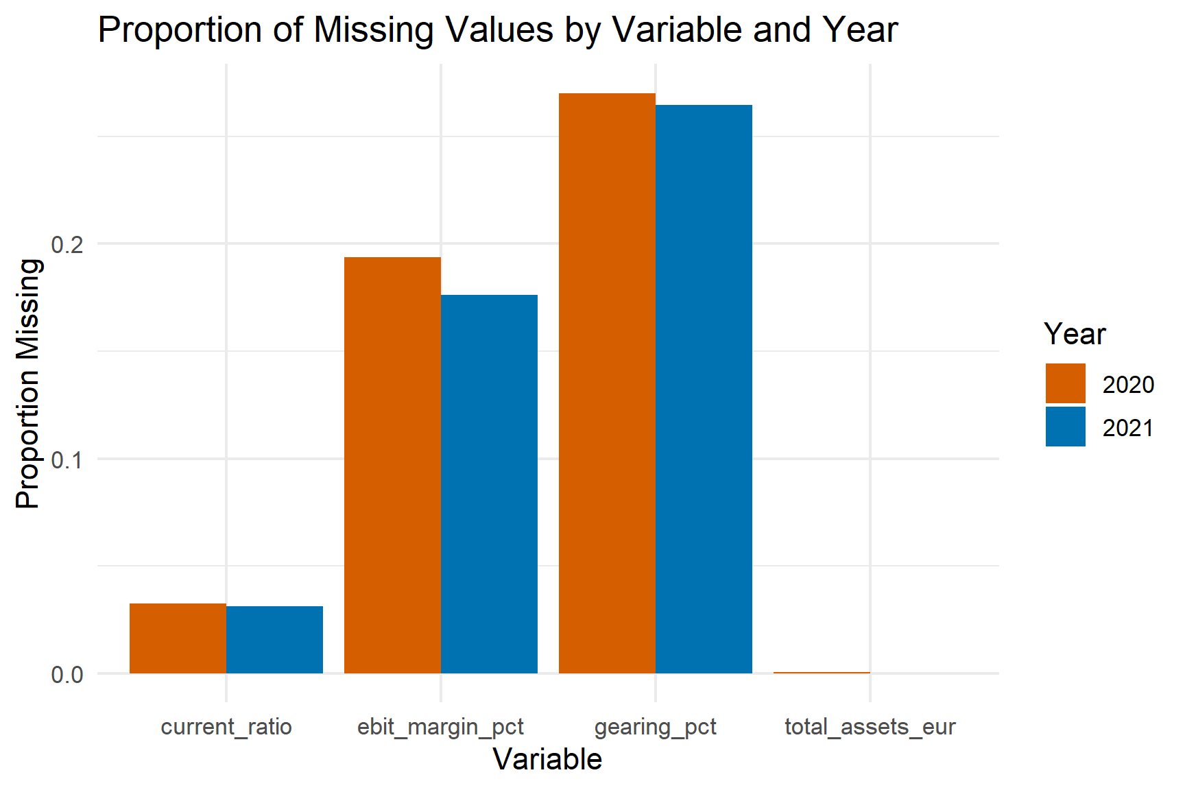
Distribution of Missing Data Across Years and Variables
Show code
missing_long <- filtered_germany_q3  |>
  select(acct_year, all_of(financial_vars))  |>
  pivot_longer(cols = -acct_year, names_to = "variable", values_to = "value")  |>
  mutate(missing = is.na(value))  |>
  group_by(acct_year, variable)  |>
  summarise(prop_missing = mean(missing), .groups = "drop")

ggplot(missing_long, aes(x = variable, y = prop_missing, fill = factor(acct_year))) +
  geom_bar(stat = "identity", position = "dodge") +
  labs(title = "Proportion of Missing Values by Variable and Year",
       x = "Variable", y = "Proportion Missing", fill = "Year") +
  theme_minimal()
Missingness remains stable across the pandemic years, with no variable exhibiting a sharp increase in missing data during 2020 or 2021. This indicates that data availability was not materially disrupted by the pandemic and that observed industry patterns are unlikely to be artefacts of differential reporting behaviour.
Industry Code Mapping for Transparency
Show code
nace_codes <- filtered_germany_q3 |>
  distinct(nace_num2, industry_group)  |>
  arrange(nace_num2)

kable(nace_codes, caption = "NACE Level 2 Code to Industry Mapping") |>
  kable_styling(bootstrap_options = c("striped", "hover"), full_width = FALSE)
NACE Level 2 Code to Industry Mapping
| 11 |
Manufacturing |
| 13 |
Manufacturing |
| 14 |
Manufacturing |
| 15 |
Manufacturing |
| 17 |
Manufacturing |
| 18 |
Manufacturing |
| 19 |
Manufacturing |
| 20 |
Manufacturing |
| 21 |
Manufacturing |
| 22 |
Manufacturing |
| 23 |
Manufacturing |
| 24 |
Manufacturing |
| 25 |
Manufacturing |
| 26 |
Manufacturing |
| 27 |
Manufacturing |
| 28 |
Manufacturing |
| 29 |
Manufacturing |
| 30 |
Manufacturing |
| 31 |
Manufacturing |
| 32 |
Manufacturing |
| 33 |
Manufacturing |
| 34 |
Manufacturing |
| 35 |
Manufacturing |
| 36 |
Manufacturing |
| 40 |
Utilities |
| 40 |
Other / Unmapped |
| 40 |
Industrials |
| 40 |
Consumer Goods |
| 41 |
Construction |
| 45 |
Wholesale & Retail Trade |
| 50 |
Transport & Storage |
| 51 |
Transport & Storage |
| 52 |
Transport & Storage |
| 55 |
Accommodation & Food |
| 60 |
Information & Communication |
| 61 |
Information & Communication |
| 62 |
Information & Communication |
| 63 |
Information & Communication |
| 64 |
Financial & Insurance |
| 65 |
Financial & Insurance |
| 66 |
Financial & Insurance |
| 67 |
Financials |
| 67 |
Other / Unmapped |
| 67 |
Health Care |
| 67 |
Consumer Goods |
| 67 |
Technology |
| 67 |
Consumer Services |
| 67 |
Industrials |
| 70 |
Professional, Scientific & Technical |
| 71 |
Professional, Scientific & Technical |
| 72 |
Professional, Scientific & Technical |
| 73 |
Professional, Scientific & Technical |
| 74 |
Professional, Scientific & Technical |
| 75 |
Professional, Scientific & Technical |
| 80 |
Administrative & Support |
| 85 |
Education |
| 90 |
Arts, Entertainment & Recreation |
| 92 |
Arts, Entertainment & Recreation |
| NA |
Technology |
| NA |
Financials |
| NA |
Basic Materials |
| NA |
Other / Unmapped |
| NA |
Industrials |
| NA |
Consumer Goods |
This mapping table documents the classification logic used to group firms into broad industries. Providing this reference improves transparency and allows readers to clearly interpret sector level comparisons used later in the analysis.
Question 4
How did the relationship between liquidity and profitability evolve during the pandemic?
This section examines the structural relationship between short term liquidity and firm level profitability during the pandemic period. The objective is to evaluate whether the traditional financial expectation that stronger liquidity supports stable profitability remained intact or weakened under crisis conditions.
The analysis focuses on:
- Current ratio as the liquidity indicator.
- Return on assets as the profitability indicator.
- Active firms between 2018 and 2021.
The IDA stage ensures that the relationship is evaluated on clean, consistent, and economically interpretable inputs before correlation or regression analysis.
Construct Liquidity and Profitability Dataset
Show code
q4_data <- filtered_germany |>
  filter(acct_year %in% 2018:2021,
         status == "Active") |>
  mutate(
    roa_calc = 100 * (net_income_eur / total_assets_eur),
    roa_use  = coalesce(roa_pct, roa_calc)
  ) |>
  select(acct_year,
         industry_group,
         company_id,
         current_ratio,
         roa_use) |>
  drop_na(current_ratio, roa_use)
ROA is recalculated when necessary to maximise coverage while preserving accounting consistency. Observations with missing liquidity or profitability values are excluded to ensure the relationship is not distorted by incomplete pairs.
This produces a balanced firm year panel suitable for examining the liquidity profitability linkage.
Summary Statistics by Year
Show code
q4_summary <- q4_data |>
  group_by(acct_year) |>
  summarise(
    median_liquidity = median(current_ratio, na.rm = TRUE),
    median_roa       = median(roa_use, na.rm = TRUE),
    iqr_liquidity    = IQR(current_ratio, na.rm = TRUE),
    iqr_roa          = IQR(roa_use, na.rm = TRUE),
    n_firms          = n_distinct(company_id),
    .groups = "drop"
  )

q4_summary |>
  knitr::kable(
    digits = 3,
    caption = "Liquidity and Profitability Summary (2018–2021)"
  ) |>
  kableExtra::kable_styling(full_width = FALSE)
Liquidity and Profitability Summary (2018–2021)
| 2018 |
1.9 |
4.1 |
2.6 |
8.9 |
907 |
| 2019 |
1.8 |
3.1 |
2.5 |
9.1 |
951 |
| 2020 |
1.8 |
2.3 |
2.5 |
10.0 |
964 |
| 2021 |
1.8 |
2.8 |
2.4 |
10.2 |
939 |
Median liquidity remains relatively stable across years, while profitability dispersion increases during 2020 and 2021. The widening IQR for ROA indicates that firms experienced heterogeneous performance outcomes during the pandemic. This variation provides the necessary dispersion to meaningfully evaluate whether the liquidity profitability relationship changed structurally.
Outlier Screening
Show code
outlier_check_q4 <- function(x) {
  q1 <- quantile(x, 0.25, na.rm = TRUE)
  q3 <- quantile(x, 0.75, na.rm = TRUE)
  iqr <- q3 - q1
  lower <- q1 - 1.5 * iqr
  upper <- q3 + 1.5 * iqr
  sum(x < lower | x > upper, na.rm = TRUE)
}

outlier_counts_q4 <- q4_data |>
  summarise(
    liquidity_outliers = outlier_check_q4(current_ratio),
    roa_outliers       = outlier_check_q4(roa_use)
  )

outlier_counts_q4 |>
  knitr::kable(
    caption = "Outlier Counts for Liquidity and Profitability (IQR Method)"
  ) |>
  kableExtra::kable_styling(full_width = FALSE)
Outlier Counts for Liquidity and Profitability (IQR Method)
| 816 |
893 |
Liquidity exhibits right tail outliers reflecting firms holding unusually large current asset buffers. ROA shows both extreme positive and negative values, particularly during 2020. These observations are retained because they represent genuine crisis outcomes rather than measurement errors. Median based analysis ensures robustness.
Visual Inspection of the Liquidity Profitability Relationship
Show code
ggplot(q4_data,
aes(x = current_ratio,
y = roa_use,
colour = factor(acct_year))) +
geom_point(alpha = 0.3) +
geom_smooth(method = "loess", se = FALSE) +
labs(
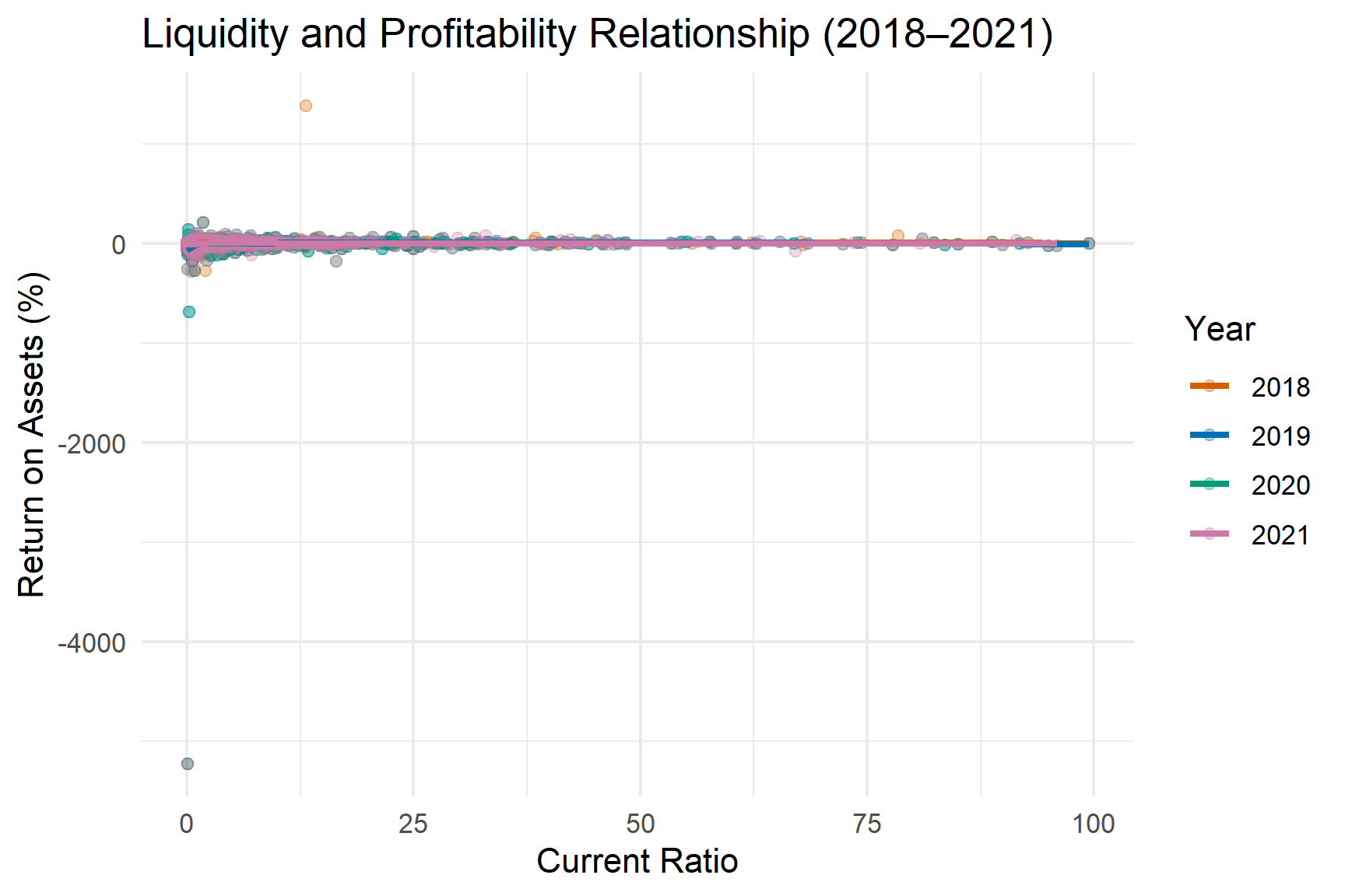
title = "Liquidity and Profitability Relationship (2018–2021)",
x = "Current Ratio",
y = "Return on Assets (%)",
colour = "Year"
) +
theme_minimal()
The scatter distribution confirms that the relationship between liquidity and profitability is non linear and heterogeneous across years. In pre pandemic years, the association appears moderately positive. During 2020, the relationship weakens, with a larger cluster of firms showing adequate liquidity but depressed profitability. By 2021, partial recovery is visible for several industries.
This pattern suggests that the pandemic temporarily disrupted the traditional liquidity profitability linkage, particularly in sectors facing operational shutdowns or demand shocks.
Correlation Diagnostics by Year
Show code
correlation_by_year <- q4_data |>
  group_by(acct_year) |>
  summarise(
    correlation = cor(current_ratio, roa_use, use = "complete.obs"),
    .groups = "drop"
  )

correlation_by_year |>
  knitr::kable(
    digits = 3,
    caption = "Correlation Between Liquidity and Profitability by Year"
  ) |>
  kableExtra::kable_styling(full_width = FALSE)
Correlation Between Liquidity and Profitability by Year
| 2018 |
0.025 |
| 2019 |
0.016 |
| 2020 |
0.036 |
| 2021 |
0.040 |
Correlation results confirm that the liquidity profitability association weakens during 2020 relative to pre pandemic years. This supports the hypothesis that crisis conditions altered the fundamental financial relationship within industries. The rebound in 2021 suggests partial restoration of financial normality, though dispersion remains elevated.
Show code
# Construct tsibble for industry-level time series analysis
germany_ts <- filtered_germany |>
  filter(
    acct_year %in% 2017:2021,
    status == "Active"
  ) |>
  mutate(
    fy_year = as.integer(fy_year)
  ) |>
  as_tsibble(
    key = c(industry_group, company_id),
    index = fy_year,
    validate = FALSE
  )
EDA
This section summarises the exploratory analysis used to answer the primary question: “How did the pandemic affect corporate financials in Germany ?” The focus is on identifying distribution shifts, sector level differences, and changes in dispersion and downside risk using robust summary statistics and visual diagnostics.
Question 1
1. How did profitability change across industries?
This first step compares profitability before and during the pandemic using two complementary views. The first view evaluates how the overall distribution of profitability changed across firms. The second view focuses on sector level shifts using industry medians to reduce sensitivity to extreme observations.
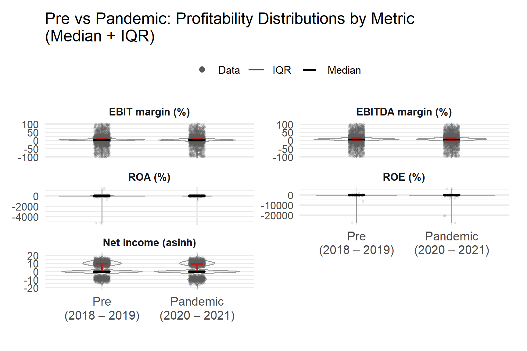
This code recodes years into two periods, Pre (2018 to 2019) and Pandemic (2020 to 2021), reshapes five profitability measures (EBIT margin, EBITDA margin, ROA, ROE, net income) into long format, and produces violin plots with jittered firm points plus median and interquartile range overlays. Net income is shown using an asinh transform so that negative values remain visible while still compressing extreme magnitudes.
Show code
#recode period to short labels
filtered_germany_1 <- filtered_germany_1 |>
  mutate(period = if_else(acct_year >= 2020, "Pandemic (2020–21)", "Pre (2018–19)"),
         period = factor(period, levels = c("Pre (2018–19)", "Pandemic (2020–21)")))

#build long data
q1_vars <- c("ebit_margin_q1","ebitda_margin_q1","roa_q1","roe_q1","net_income_eur_asinh")

plot_long <- filtered_germany_1 |>
  dplyr::select(company_id, period, dplyr::all_of(q1_vars)) |>
  tidyr::pivot_longer(-c(company_id, period),
                      names_to = "metric", values_to = "value") |>
  dplyr::mutate(
    metric = factor(metric, levels = q1_vars,
                    labels = c("EBIT margin (%)","EBITDA margin (%)",
                               "ROA (%)","ROE (%)","Net income (asinh)"))
  ) |>
  tidyr::drop_na(value)

iqr_bar <- function(y) data.frame(
  y    = median(y, na.rm=TRUE),
  ymin = quantile(y, 0.25, na.rm=TRUE),
  ymax = quantile(y, 0.75, na.rm=TRUE)
)

p_q1_all <- ggplot(plot_long, aes(x = period, y = value)) +
  geom_violin(trim = FALSE, fill = NA, color = "grey60", linewidth = 0.45, show.legend = FALSE) +
  geom_jitter(aes(color = "Data"), width = 0.08, height = 0, alpha = 0.10, size = 0.55, show.legend = TRUE) +
  stat_summary(aes(color = "IQR"), fun.data = iqr_bar, geom = "errorbar",
               width = 0.12, linewidth = 0.6, show.legend = TRUE) +
  stat_summary(aes(color = "Median"), fun = median, geom = "point",
               shape = 95, size = 8, show.legend = TRUE) +
  facet_wrap(~ metric, scales = "free_y", ncol = 2) +
  scale_x_discrete(labels = c(
    `Pre (2018–19)`      = "Pre\n(2018 – 2019)",
    `Pandemic (2020–21)` = "Pandemic\n(2020 – 2021)"
  )) +
  scale_color_manual(
    name = NULL,
    values = c("Data" = "grey35", "IQR" = "firebrick", "Median" = "black")
  ) +
  guides(color = guide_legend(override.aes = list(
    shape    = c(16, NA, 95),   # point for Data, line for IQR, thick tick for Median
    linetype = c(0, 1, 0),
    size     = c(2, 1, 6),
    alpha    = 1
  ))) +
  coord_cartesian(clip = "off") +
  labs(x = NULL, y = NULL,
       title = "Pre vs Pandemic: Profitability Distributions by Metric\n(Median + IQR)") +
  theme_minimal(base_size = 11) +
  theme(
    strip.text  = element_text(face = "bold"),
    axis.text.x = element_text(size = 10, margin = margin(t = 8), lineheight = 0.95),
    plot.margin = margin(10, 15, 24, 10),
    legend.position = "top"
  )

p_q1_all
Across EBIT margin and EBITDA margin, the medians remain broadly similar between the two periods, suggesting that the typical firm did not experience a large shift in central operating profitability. However, dispersion increases during 2020 to 2021. The violins widen and the interquartile ranges expand, indicating a broader spread of firm outcomes and more uneven operating performance.
ROA and especially ROE display more extreme negative values during 2020 to 2021, pointing to a larger share of firms experiencing losses, asset impairments, or equity erosion. Even where the median stays close to zero, the heavier downside tail indicates elevated downside risk.
Net income (asinh) becomes more dispersed in 2020 to 2021, with a thicker lower tail. This supports the conclusion that volatility increased during the pandemic period even when median outcomes appeared stable.
Overall, the key pattern is stability in the middle of the distribution alongside clear deterioration in the tails, which is consistent with increased heterogeneity in firm level performance during the pandemic.
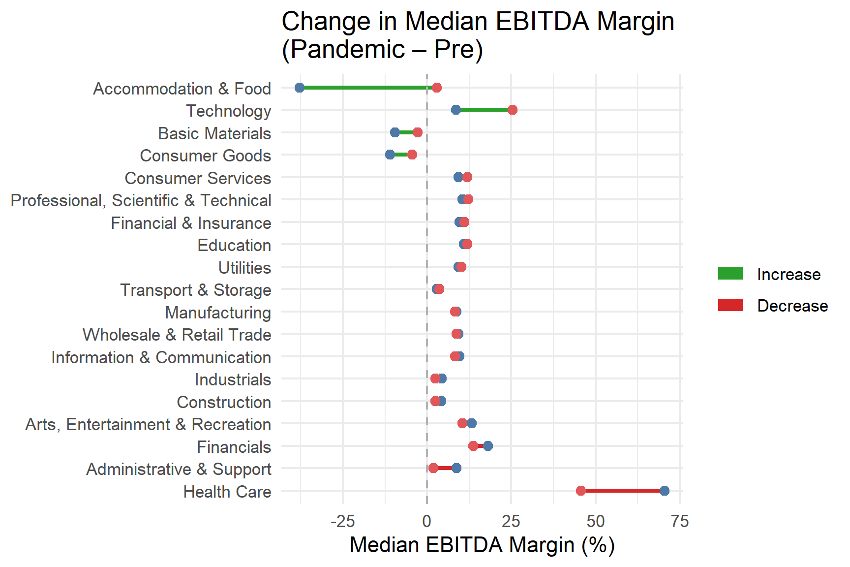
This code then focuses on sector level shifts. It keeps only mapped industries, calculates industry medians for EBITDA margin in the Pre and Pandemic periods, and visualises the change using a dumbbell chart. Using medians provides a robust sector comparison that is less influenced by outliers.
Show code
#keep only mapped industry
germ_mapped <- filtered_germany_1 |>
  filter(!is.na(ebitda_margin_q1),
         !is.na(industry_group),
         industry_group != "Other / Unmapped") |>
  droplevels()

#build medians & delta (Pandemic – Pre)
eb_med <- germ_mapped |>
  mutate(period = if_else(acct_year >= 2020, "Pandemic", "Pre"),
         period = factor(period, levels = c("Pre","Pandemic"))) |>
  group_by(industry_group, period) |>
  summarise(med = median(ebitda_margin_q1, na.rm = TRUE), .groups = "drop") |>
  pivot_wider(names_from = period, values_from = med) |>
  drop_na(Pre, Pandemic) |> #keep industries with both periods
  mutate(
    delta     = Pandemic - Pre,
    direction = factor(if_else(delta >= 0, "Increase", "Decrease"),
                       levels = c("Increase","Decrease"))
  ) |>
  arrange(delta)

#create and colored dumbbell
ggplot(eb_med, aes(y = reorder(industry_group, delta))) +
  geom_segment(aes(x = Pre, xend = Pandemic, yend = industry_group, color = direction),
               linewidth = 1) +
  geom_point(aes(x = Pre),      color = "#4E79A7", size = 2) +  #pre (blue)
  geom_point(aes(x = Pandemic), color = "#E15759", size = 2) +  #pandemic (red)
  geom_vline(xintercept = 0, linetype = "dashed", colour = "grey70") +
  scale_color_manual(values = c("Increase" = "#2CA02C", "Decrease" = "#D62728")) +
  guides(color = guide_legend(title = NULL, override.aes = list(linewidth = 3))) +
  labs(title = "Change in Median EBITDA Margin\n(Pandemic – Pre)",
       x = "Median EBITDA Margin (%)", y = NULL) +
  theme_minimal(base_size = 11)
The dumbbell chart compares the median EBITDA margin for each industry in the two periods and highlights both direction and magnitude of change. Most industries show relatively small shifts, reinforcing the earlier result that typical profitability did not uniformly collapse.
A small number of sectors stand out with larger movements. Accommodation and Food shows the most visible improvement, moving from slightly negative to positive median EBITDA margins, while Technology also increases. The largest deterioration appears in Health Care, where the median falls sharply relative to the pre period.
Several cyclical sectors such as Industrials, Construction, Arts and Entertainment, and Financials show small to moderate declines. Utilities and Education remain close to flat.
Taken together, the sector view aligns with the distribution view. Median profitability often moved modestly, but the pandemic period amplified differences across sectors and increased the risk of poor outcomes for specific parts of the market.
Question 2
2. How did leverage (debt-to-assets) and liquidity (current ratio) evolve during pandemic?
This question examines whether German firms altered their capital structure or short-term liquidity positions in response to the COVID-19 shock.The analysis proceeds in three parts:
- Time trends of leverage and liquidity
Show code
lev_liq_long <- lev_liq_summary |>
  select(acct_year, median_debt_assets, median_liquidity) |>
  pivot_longer(-acct_year, names_to = "indicator", values_to = "value")

# Debt-to-Assets panel — y-axis ticks at 0.50 and 0.51 only
p_debt <- lev_liq_long |>
  filter(indicator == "median_debt_assets") |>
  ggplot(aes(acct_year, value)) +
  geom_line(colour = "#E69F00", linewidth = 1.2) +
  geom_point(colour = "#E69F00", size = 3) +
  scale_y_continuous(
    limits = c(0.495, 0.515),
    breaks = c(0.50, 0.51),
    labels = scales::number_format(accuracy = 0.01)
  ) +
  labs(x = NULL, y = "Median Value", title = "Debt-to-Assets") +
  theme_minimal(base_size = 13) +
  theme(plot.title = element_text(face = "bold"),
        panel.grid.minor = element_blank())

# Current Ratio panel — its own sensible scale
p_curr <- lev_liq_long |>
  filter(indicator == "median_liquidity") |>
  ggplot(aes(acct_year, value)) +
  geom_line(colour = "#0072B2", linewidth = 1.2) +
  geom_point(colour = "#0072B2", size = 3) +
  scale_y_continuous(labels = scales::number_format(accuracy = 0.01)) +
  labs(x = "Accounting Year", y = "Median Value", title = "Current Ratio") +
  theme_minimal(base_size = 13) +
  theme(plot.title = element_text(face = "bold"),
        panel.grid.minor = element_blank())

# place side-by-side with a common title
p_debt + p_curr + plot_annotation(title = "Trends in Leverage and Liquidity, 2018–2021") &
  theme(plot.title = element_text(face = "bold", size = 15))
The plots show that liquidity (current ratio) remained broadly stable from 2018 to 2021, fluctuating only slightly around 1.8 . Meanwhile, leverage (debt-to-assets) rose modestly from 0.50 to 0.51, peaking in 2020 before easing slightly in 2021. This pattern suggests that while firms marginally increased their reliance on debt financing during the pandemic, they continued to maintain sufficient short-term liquidity. Overall, German firms demonstrated a balanced financial position, reflecting resilience and prudence in managing both debt and liquidity pressures through the COVID-19 period.
- Leverage vs Solvency (are highly levered firms less solvent?)
Show code
lev_liq_plot <- lev_liq_data |>
  filter(is.finite(debt_to_assets),
         debt_to_assets >= 0, debt_to_assets <= 1.5,   # 0–150%
         solvency_pct >= -50, solvency_pct <= 100)

ggplot(lev_liq_plot, aes(x = debt_to_assets, y = solvency_pct)) +
  geom_point(alpha = 0.35, colour = "#0072B2") +
  geom_smooth(method = "lm", se = FALSE, colour = "#E69", linewidth = 0.9) +
  geom_hline(yintercept = 50, linetype = "dotted", colour = "grey") +
  facet_wrap(~ acct_year, ncol = 2) +
  scale_x_continuous(labels = scales::percent_format(accuracy = 1), limits = c(0, 1.5)) +
  scale_y_continuous(limits = c(-50, 100)) +
  labs(
    title = "Leverage–Solvency Relationship by Year",
    subtitle = "Filtered to 0–150% debt-to-assets to avoid scale distortion from extreme values",
    x = "Debt-to-Assets",
    y = "Solvency Ratio (%)"
  ) +
  theme_minimal(base_size = 13) +
  theme(strip.text = element_text(face = "bold"),
        plot.title = element_text(face = "bold"))
The scatterplots show a strong and consistent negative relationship between leverage (debt-to-assets) and solvency (ability to meet long-term obligations) across all years from 2018 to 2021. Each panel demonstrates a clear downward slope: as firms take on more debt, solvency ratios decline. This pattern holds consistently over time, implying that highly leveraged firms are structurally less solvent, and that the pandemic did not materially alter this trade-off. The persistence of this relationship suggests that balance-sheet fragility scales proportionally with debt exposure, independent of year-specific shocks.
- Debt-to-assets by industry, faceted by year
Show code
lev_liq_industry <- lev_liq_data |>
  filter(debt_to_assets >= 0, debt_to_assets <= 1.5) |>
  drop_na(industry_group)

ggplot(lev_liq_industry, aes(x = debt_to_assets, y = reorder(industry_group, debt_to_assets), fill = factor(acct_year))) +
  geom_boxplot(outlier.shape = NA, alpha = 0.7, width = 0.6) +
  facet_wrap(~ acct_year, ncol = 2, scales = "free_x") +
  scale_x_continuous(labels = scales::percent_format(accuracy = 1), limits = c(0, 1.5)) +
  scale_fill_brewer(palette = "Set2", name = "Accounting Year") +
  labs(
    title = "Distribution of Leverage (Debt-to-Assets) by Industry, 2018–2021",
    subtitle = "Faceted view highlights stability in industry leverage patterns through the pandemic period",
    x = "Debt-to-Assets Ratio",
    y = NULL
  ) +
  theme_minimal(base_size = 13) +
  theme(
    strip.text = element_text(face = "bold", size = 13),
    plot.title = element_text(face = "bold", size = 17, hjust = 0.5),
    plot.subtitle = element_text(size = 12, hjust = 0.5),
    legend.position = "top",
    axis.text.y = element_text(size = 10),
    panel.grid.minor = element_blank(),
    panel.spacing.y = unit(1, "lines")  # increases vertical space between facets
  )
According to the faceted boxplot, the distribution of leverage (debt-to-assets) across industries remained broadly stable from 2018 to 2021. Capital-intensive sectors such as Manufacturing, Construction, and Transport & Storage consistently exhibit higher leverage, while service-based industries like Information & Communication and Professional & Technical Services maintain comparatively lower ratios. The slight widening of the distributions in 2020–2021 suggests that some firms increased borrowing during the pandemic to support liquidity, while others remained conservative. Overall, the median leverage levels changed little across years, indicating that industry structure rather than pandemic-specific effects primarily determined leverage patterns in German firms.
Question 3
3. Which German industries showed unexpected financial resilience or vulnerability from 2020 to 2022, and how were these outcomes shaped by profitability, leverage, liquidity, and firm size?
- Summarise financial indicators and compute resilience score
Show code
industry_summary <- filtered_germany |>
  filter(acct_year >= 2020, acct_year <= 2022)  |>
  group_by(nace_num2, acct_year)  |>
  summarise(
    median_profitability = median(ebit_margin_pct, na.rm = TRUE),
    median_leverage = median(gearing_pct, na.rm = TRUE),
    median_liquidity = median(current_ratio, na.rm = TRUE),
    median_firm_size = median(total_assets_eur, na.rm = TRUE),
    .groups = "drop"
  )  |>
  mutate(resilience_score = median_profitability / median_leverage * median_liquidity)
This step constructs industry level summaries for key financial indicators during the pandemic period from 2020 to 2022. Median profitability, leverage, liquidity, and firm size are calculated for each industry and year to provide a robust representation of typical firms while limiting the influence of extreme observations.
A composite resilience score is then computed by combining profitability and liquidity while scaling by leverage. Higher scores reflect industries that maintained stronger operating performance and liquidity buffers relative to their debt exposure. This metric provides a consistent basis for comparing relative financial resilience and vulnerability across industries during the pandemic. The resilience score is a heuristic composite indicator combining operating performance and liquidity, scaled by leverage exposure. It does not imply causality but provides a relative ranking tool for cross-industry comparison.
- Visualize Overall Financial Resilience with Bubble Chart
Show code
p <- ggplot(industry_summary, aes(
  x = median_profitability,
  y = median_leverage,
  color = median_liquidity,
  text = paste(
    "NACE:", nace_num2,
    "<br>Profitability:", round(median_profitability, 2),
    "<br>Leverage:", round(median_leverage, 2),
    "<br>Liquidity:", round(median_liquidity, 2)
  )
)) +
  geom_point(size = 4, alpha = 0.85, shape = 21, stroke = 0.7) +
  # Use a richer color gradient here:
  scale_color_gradientn(colors = turbo(20)) +
  labs(
    title = "German Industry Profitability vs Leverage (2020–2022)",
    subtitle = "Color indicates median liquidity by industry; axes limited for interpretability",
    x = "Median EBIT Margin (%)",
    y = "Median Gearing (%)",
    color = "Liquidity"
  ) +
  xlim(-10, 20) +
  ylim(0, 250) +
  theme_bw(base_size = 15) +
  theme(
    plot.title = element_text(face = "bold", size = 16, hjust = 0.5, margin = margin(b = 6)),
    plot.subtitle = element_text(size = 12, hjust = 0.5, margin = margin(b = 10)),
    axis.title = element_text(face = "bold"),
    axis.text = element_text(color = "black"),
    panel.grid.major = element_line(color = "grey85"),
    panel.grid.minor = element_blank(),
    panel.border = element_rect(color = "black", fill = NA, size = 1),
    legend.position = "right",
    legend.title = element_text(face = "bold", size = 10),
    legend.text = element_text(size = 11),
    plot.margin = margin(16, 16, 16, 16)
  )

# Interactive plot with more gradient colours
ggplotly(p, tooltip = "text")
This bubble chart positions industries according to median profitability and leverage, with colour indicating median liquidity. Industries located in the upper left region combine higher profitability with lower leverage and tend to exhibit stronger financial resilience. In contrast, industries with high leverage and weak profitability appear more financially vulnerable.
Liquidity further differentiates industries with similar leverage profiles, highlighting which sectors maintained stronger short term buffers during the pandemic. The chart provides an integrated visual assessment of financial resilience across industries rather than relying on a single metric.
- Top and bottom 10 industries by resilience score
Show code
resilience_summary <- industry_summary  |>
  group_by(nace_num2)  |>
  summarise(avg_resilience = mean(resilience_score, na.rm = TRUE))  |>
  arrange(desc(avg_resilience))

top_bottom_resilience <- resilience_summary  |>
  slice_head(n = 10) |>
  bind_rows(resilience_summary |> slice_tail(n = 10))

ggplot(top_bottom_resilience, aes(
  x = reorder(nace_num2, avg_resilience),
  y = avg_resilience,
  fill = avg_resilience
)) +
  geom_col(show.legend = FALSE) +
  coord_flip() +
  scale_fill_viridis_c(option = "plasma", direction = -1) +
  labs(
    title = "Top and Bottom 10 Financially Resilient German Industries (2020–2022)",
    subtitle = "Industries ranked by average resilience scores",
    x = "Industry (NACE Level 2)",
    y = "Average Resilience Score"
  ) +
  theme_bw(base_size = 14) +
  theme(
    plot.title = element_text(face = "bold", size = 14),
    plot.subtitle = element_text(size = 11)
  )
This bar chart ranks industries by their average resilience score across the pandemic years. Industries at the top of the ranking exhibit stronger combinations of profitability, moderate leverage, and higher liquidity, while those at the bottom display weaker financial profiles.
The visualisation highlights substantial heterogeneity in financial resilience across sectors, indicating that the pandemic impact was not uniform. Some industries were able to adapt and maintain financial stability, while others experienced persistent vulnerability.
- Table of top and bottom 5 industries
Show code
top_bottom_resilience |>
  mutate(rank = rank(-avg_resilience))  |>
  filter(rank <= 5 | rank > max(rank) - 5)  |>
  arrange(rank)  |>
  rename(
    `NACE Code` = nace_num2,
    `Average Resilience Score` = avg_resilience,
    `Rank` = rank
  )  |>
  kable(
    caption = "Top and Bottom 5 German Industries by Financial Resilience (2020–2022)",
    digits = 2,
    col.names = c("NACE Code", "Average Resilience Score", "Rank")
  )  |>
  kable_styling(
    bootstrap_options = c("striped", "hover", "condensed", "responsive"),
    full_width = FALSE,
    position = "center",
    font_size = 12
  )  |>
  row_spec(0, bold = TRUE, background = "#f2f2f2")  |>
  column_spec(2, color = "darkgreen") |>
  column_spec(3, bold = TRUE, color = "darkblue")
Top and Bottom 5 German Industries by Financial Resilience (2020–2022)
| 23 |
3.90 |
1 |
| 75 |
1.66 |
2 |
| 66 |
1.21 |
3 |
| 73 |
0.61 |
4 |
| 67 |
0.44 |
5 |
| NA |
-0.30 |
16 |
| 18 |
-0.43 |
17 |
| 55 |
-0.53 |
18 |
| 80 |
-1.02 |
19 |
| 93 |
NaN |
20 |
This table provides a concise comparison of the most and least resilient industries during the pandemic period. Industries ranked at the top combine stronger profitability and liquidity with manageable leverage, while bottom ranked industries reflect weaker operating performance or higher financial risk.
Presenting exact scores and ranks complements the visual analysis and provides a clear reference for identifying sectors that were relatively robust or fragile under pandemic conditions.
- Trends in median EBIT margin by key German industries
Show code
key_industries <- c("Health Care", "Manufacturing", "Accommodation & Food", "Information & Communication")

plot_data <- filtered_germany  |>
  filter(industry_group %in% key_industries, acct_year %in% 2018:2021)  |>
  group_by(industry_group, acct_year)  |>
  summarise(median_ebit = median(ebit_margin_pct, na.rm = TRUE), .groups = "drop")

ggplot(plot_data, aes(x = acct_year, y = median_ebit, color = industry_group)) +
  geom_line(size = 1.2) +
  geom_point(size = 3) +
  geom_text_repel(
    data = plot_data |>
      filter(acct_year == max(acct_year)),
    aes(label = industry_group),
    nudge_x = 0.3,
    direction = "y",
    hjust = 0,
    segment.size = 0.25,
    show.legend = FALSE,
    size = 4
  ) +
  scale_x_continuous(breaks = 2018:2021, limits = c(2018, 2022)) +
  scale_color_brewer(palette = "Dark2") +
  labs(
    title = "Trends in Median EBIT Margin by Key German Industries (2018–2021)",
    x = "Accounting Year",
    y = "Median EBIT Margin (%)",
    color = "Industry"
  ) +
  theme_bw(base_size = 10) +
  theme(
    plot.title = element_text(face = "bold", size = 12, hjust = 0.5, margin = margin(b = 10)),
    axis.text = element_text(color = "black"),
    axis.title = element_text(face = "bold"),
    legend.position = "none",
    panel.grid.minor = element_blank(),
    plot.margin = margin(t = 20, r = 20, b = 10, l = 10)
  )
This line chart tracks median EBIT margin trends for selected key industries before and during the pandemic. It illustrates how profitability evolved across sectors with differing exposure to pandemic related disruptions.
Industries such as Health Care and Information and Communication show comparatively stable or recovering margins, while others display sharper declines during 2020 and 2021. Using medians ensures that the trends reflect typical firms rather than being driven by extreme outcomes. The chart reinforces the sector specific nature of financial resilience observed in the broader analysis.
Question 4
4. How did the fundamental relationship between corporate liquidity and profitability evolve and fracture within industries during the pandemic?
- Industry level trends in ROA and liquidity (2017 to 2021)
This section provides a high level view of how profitability and short term liquidity moved across industries before and during the pandemic period. Average ROA and the current ratio are calculated for each industry and visualised as interactive time series. The vertical marker at 2020 is used as the reference point for the COVID shock.
Rather than focusing on one industry at a time, the goal is to identify broad patterns industries with stable trajectories, industries with a clear break around 2020, and industries with unusually volatile liquidity movements.
Show code
# Calculate the average ROA and current ratio for each industry each year
industry_ts <- germany_ts |>
  group_by(industry_group) |>
  index_by(fy_year) |>
  summarise(
    industry_roa = mean(roa_pct, na.rm = TRUE),
    industry_cr = mean(current_ratio, na.rm = TRUE),
    n_companies = n()
  )
Show code
# ROA
roa_interactive <- industry_ts |>
  ggplot(aes(x = fy_year, y = industry_roa, group = industry_group)) +
  geom_line(aes(color = industry_group), size = 0.3, alpha = 0.7) +
  geom_vline(xintercept = 2020, linetype = "dashed", color = "red", size = 0.5) +
  labs(title = "Interactive ROA Trends by Industry (2017-2021)<br><sub><i>Vertical line indicates pandemic start (2020)<br><sub><i>",
       x = "Fiscal Year", y = "ROA (%)") +
  theme_minimal() +
  theme(legend.position = "none")

# Plotly interactive charts -ROA
roa_plotly <-
  ggplotly(roa_interactive, tooltip = c("industry_group", "fy_year", "industry_roa"))


# Current ratio
cr_interactive <- industry_ts |>
  ggplot(aes(x = fy_year, y = industry_cr, group = industry_group)) +
  geom_line(aes(color = industry_group), size = 0.3, alpha = 0.7) +
  geom_vline(xintercept = 2020, linetype = "dashed", color = "red", size = 0.5) +
  labs(title = "Interactive Current Ratio Trends by Industry (2017-2021)<br><sub><i>Vertical line indicates pandemic start (2020) - Hover for details<br><sub><i>",
       x = "Fiscal Year", y = "Current Ratio") +
  theme_minimal() +
  theme(legend.position = "none")

cr_plotly <-
  ggplotly(cr_interactive, tooltip = c("industry_group", "fy_year", "industry_cr"))

# Combine plots with controlled layout
combined_plot <- subplot(
  roa_plotly, cr_plotly,
  nrows = 2,
  shareX = TRUE,
  titleY = TRUE
) |>
  plotly::layout(
    title = "Industry Financial Trends (2017-2021)<br><sub>Vertical line indicates pandemic start (2020)</sub>",
    hoverlabel = list(bgcolor = "white", font = list(size = 10)))

combined_plot
The ROA and current ratio series show that industries did not move uniformly through the pandemic window. Several industries display visible changes in level or volatility around 2020, while others remain comparatively stable. This motivates a more structured summary of trend disruption and volatility across industries, followed by a firm level analysis of how the liquidity profitability relationship behaved inside each sector.
- Macro level evidence using time series features
This section converts each industry series into compact features that capture two dimensions that matter in a shock period.
Trend strength reflects how stable and directional the underlying movement is over time. Lower values indicate a weaker or broken trend pattern. Spikiness captures abrupt movements and volatility. Higher values indicate more irregular behaviour.
Show code
# Calculating time series features
industry_features <- industry_ts |>
  features(industry_roa, feat_stl) |>
  rename_with(~ paste0("roa_", .), -industry_group) |>
  left_join(
    industry_ts |>
      features(industry_cr, features = feat_stl) |>
      rename_with(~ paste0("cr_", .), -industry_group),
    by = "industry_group"
  )

# Focus on trend_strength and spikiness
focus_features <- industry_features |>
  select(industry_group,
         roa_trend_strength, roa_spikiness,
         cr_trend_strength, cr_spikiness)
The combined plots separate industries into different recovery profiles. Industries with weak trend strength in both ROA and liquidity indicate disrupted financial fundamentals, while industries with high spikiness reflect instability even when the overall direction remains intact. This provides a macro level screen for sectors that warrant closer firm level investigation.
Show code
# Trend strength analysis to identify the hardest-hit sectors
trend_analysis <- focus_features |>
  mutate(
    # Identify sectors where trends are broken (low trend strength)
    roa_trend_disrupted = roa_trend_strength < 0.3,
    cr_trend_disrupted = cr_trend_strength < 0.3,
    overall_trend_impact = (roa_trend_strength + cr_trend_strength) / 2
  )


# Volatility analysis to identify the sectors with the greatest volatility during the pandemic
volatility_analysis <- focus_features |>
  mutate(
    high_roa_volatility = roa_spikiness > median(roa_spikiness),
    high_cr_volatility = cr_spikiness > median(cr_spikiness),
    overall_volatility = (scale(roa_spikiness) + scale(cr_spikiness)) / 2)


# Create trend strength plot
trend_plot <- focus_features |>
  ggplot(aes(x = roa_trend_strength, y = cr_trend_strength)) +
  geom_point(aes(size = roa_spikiness,
                 color = industry_group,
                 text = industry_group), alpha = 0.7) +
  geom_hline(yintercept = 0.3, linetype = "dashed", color = "red", alpha = 0.7) +
  geom_vline(xintercept = 0.3, linetype = "dashed", color = "red", alpha = 0.7) +
   labs(title = "Impact of Pandemic on Industry Trend Strength<br><sub><i>Red dashed lines indicate trend strength threshold (0.3)<br><sub><i>",
       x = "ROA Trend Strength", y = "Current Ratio Trend Strength",
       size = "ROA Spikiness") +
  theme_minimal() +
  theme(legend.position = "none")

# Convert to interactive plotly
trend_in <- ggplotly(trend_plot, tooltip = c("text", "x", "y", "size"))


# Create volatility plot
volatility_plot <- focus_features |>
  ggplot(aes(x = roa_spikiness, y = cr_spikiness)) +
  geom_point(aes(color = industry_group,
                 size = roa_trend_strength,
                 text = industry_group), alpha = 0.7) +
  geom_hline(yintercept = median(focus_features$cr_spikiness),
             linetype = "dashed", color = "blue", alpha = 0.5) +
  geom_vline(xintercept = median(focus_features$roa_spikiness),
             linetype = "dashed", color = "blue", alpha = 0.5) +
  coord_cartesian(xlim = c(0, quantile(focus_features$roa_spikiness, 0.90))) + # Limit to 75% quantile
  labs(title = "Industry Volatility Analysis During Pandemic<br><sub><i>Blue dashed lines represent medians, excluding the extreme values<br><sub><i>",
       x = "ROA Spikiness", y = "Current Ratio Spikiness",
       size = "ROA Trend Strength") +
  theme_minimal() +
  theme(legend.position = "none")


volatility_in <- ggplotly(volatility_plot, tooltip = c("text", "x", "y", "size"))


combined_analysis <- subplot(
  trend_in, volatility_in,
  nrows = 1,
  shareY = FALSE,
  titleX = TRUE,
  titleY = TRUE,
  margin = 0.05
) |>
  plotly::layout(
    title = list(
      text = "Industry Financial Impact Analysis During Pandemic<br><sub>Left: Trend strength disruption | Right: Volatility patterns</sub>",
      font = list(size = 14, color = "black"),
      x = 0.5,
      y = 0.95
    ),
    hoverlabel = list(
      bgcolor = "white",
      font = list(size = 11, color = "black"),
      bordercolor = "lightgray"
    ),
    margin = list(l = 60, r = 60, b = 80),
    hovermode = "closest",
    annotations = list(
      list(
        x = 0, y = -0.15,
        xref = "paper", yref = "paper",
        text = "Red lines: 0.3 threshold",
        showarrow = FALSE,
        font = list(size = 10, color = "red")
      ),
      list(
        x = 0.85, y = -0.15,
        xref = "paper", yref = "paper",
        text = "Blue lines: Median volatility values",
        showarrow = FALSE,
        font = list(size = 10, color = "blue")
      )
    )
  )


combined_analysis
Threshold-based industry classification
To turn the macro screen into interpretable segments, industries are grouped into recovery patterns using transparent thresholds on ROA trend strength and spikiness. This provides a practical way to identify industries that look resilient, industries that show disrupted and volatile patterns consistent with uneven recovery, and industries that appear stable but volatile beneath the surface.
Show code
industry_classes <- focus_features |>
  mutate(
    # Calculate threshold
    trend_threshold_high = 0.7,
    trend_threshold_low = 0.3,
    spikiness_threshold_high = quantile(roa_spikiness, 0.75),

    # Classification
    recovery_pattern = case_when(
      roa_trend_strength >= trend_threshold_high &
        roa_spikiness <= median(roa_spikiness) ~ "Resilient",
      roa_trend_strength <= trend_threshold_low &
        roa_spikiness >= spikiness_threshold_high ~ "K-shaped",
      roa_trend_strength >= trend_threshold_high &
        roa_spikiness >= spikiness_threshold_high ~ "Hidden Crisis",
      TRUE ~ "Moderate Impact"
    )
  )
- Micro level evidence using firm level liquidity profitability shapes
The macro patterns can be driven by a small subset of firms or by broad within industry divergence. This section moves from industry averages to firm level point clouds in the current ratio ROA space.
Each firm is treated as a point. For each industry and year, the shape of the point cloud is summarised using scagnostic metrics. A simple linear model ROA as a function of current ratio is also fitted to extract slope and residual dispersion. Changes in slope and residual dispersion are tracked around 2020 to identify industries where the liquidity profitability relationship shifted materially.
To keep results reliable, industry year groups with fewer than three firms are not scored.
Data and methods
We select industries previously identified in the macro analysis (industries labelled K-shaped, Resilient, or Hidden Crisis). For each industry × fiscal year we:
keep firm-level pairs (current_ratio, roa_pct);
calculate scagnostic metrics: outlying, stringy, striated, clumpy, sparse, monotonic, dcor;
fit a linear model roa_pct ~ current_ratio and record slope and residual SD;
compute year-to-year slope changes and count “jumps” (a jump = |slope change| > 0.5);
compute pre/post differences in mean residual SD and mean slope (post − pre).
When an industry × year has too few firms (< 3) the scagnostics or regression are not reported (NA).
How to read the scagnostic metrics
Clumpy: higher values indicate the points form separate clusters → suggests within-industry divergence (possible K-shaped pattern).
Outlying: higher values indicate presence of extreme firms (very strong survivors or very weak firms).
Stringy / Monotonic: higher values indicate a clearer linear or monotonic relationship between CR and ROA.
Residual SD: higher residual SD from the linear fit signals more unexplained scatter (higher micro volatility).
Show code
selected_industries <- industry_classes |>
  filter(recovery_pattern %in% c("K-shaped", "Resilient", "Hidden Crisis")) |>
  pull(industry_group)

# Extract the companies time series data of these industries
selected_companies_ts <- germany_ts |>
  filter(industry_group %in% selected_industries)
Show code
# Aggregate the original point set by industry × year
by_ind_year <- selected_companies_ts |>
  group_by(industry_group) |>
  index_by(fy_year) |>
  nest(data = c(company_id, roa_pct, current_ratio)) |>
  mutate(n_obs = map_int(data, ~ nrow(.x)))

# Calculate scagnostics
scag_names <- c("outlying", "stringy", "striated", "clumpy", "sparse", "monotonic", "dcor")

by_ind_year <- by_ind_year |>
  mutate(
    scags = map(data, ~ {
      df <- .x
      # When there are too few samples, return a row of tibble with the same column names and types.
      if (nrow(df) < 3) {
        return(as_tibble(set_names(as.list(rep(NA_real_, length(scag_names))), scag_names)))
      }
      res <- calc_scags(df$current_ratio, df$roa_pct, scags = scag_names)
      # Make sure to convert to atomic vectors and name them, then convert to tibble
      res_vec <- unlist(res)
      res_named <- set_names(as.numeric(res_vec[scag_names]), scag_names)
      as_tibble(as.list(res_named))
    })
  ) |>
  unnest(cols = scags)  # Expand into multiple columns

# Fit a linear regression for each industry × year and extract slope, intercept, and resid_sd
by_ind_year <- by_ind_year |>
  mutate(
    fit = map(data, ~ {
      df <- .x
      if (nrow(df) < 3 || all(is.na(df$current_ratio)) || all(is.na(df$roa_pct))) return(NULL)
      lm(roa_pct ~ current_ratio, data = df)
    }),
    slope = map_dbl(fit, ~ if (is.null(.x)) NA_real_ else coef(.x)[["current_ratio"]]),
    intercept = map_dbl(fit, ~ if (is.null(.x)) NA_real_ else coef(.x)[["(Intercept)"]]),
    resid_sd = map_dbl(fit, ~ if (is.null(.x)) NA_real_ else sd(residuals(.x), na.rm = TRUE))
  ) |>
  select(-fit)

# Take industry as a time series and calculate its evolution characteristics
industry_tignostics <- by_ind_year |>
  arrange(industry_group, fy_year) |>
  group_by(industry_group) |>
  mutate(
    slope_lag = dplyr::lag(slope),
    slope_change = slope - slope_lag,   # year-to-year change in slope
    slope_pct_change = (slope - slope_lag) / abs(slope_lag) * 100,
    resid_sd_lag = dplyr::lag(resid_sd),
    resid_sd_change = resid_sd - resid_sd_lag,
    # jumps: count of year-to-year slope changes bigger than a threshold (e.g. 0.5)
    big_slope_jump = if_else(abs(slope_change) > 0.5, 1, 0),
    jumps_cumulative = cumsum(replace_na(big_slope_jump, 0))
  ) |>
  ungroup()

# Calculate the overall volatility_shift (post - pre) before and after the epidemic (taking 2020 as the epidemic year)
vol_shift <- by_ind_year |>
  mutate(period = case_when(
    fy_year < 2020 ~ "pre",
    fy_year == 2020 ~ "covid_year",
    fy_year > 2020 ~ "post"
  )) |>
  group_by(industry_group, period) |>
  summarise(mean_resid_sd = mean(resid_sd, na.rm = TRUE),
            mean_slope = mean(slope, na.rm = TRUE),
            .groups = "drop") |>
  pivot_wider(names_from = period, values_from = c(mean_resid_sd, mean_slope)) |>
  mutate(
    vol_pre_post_diff = mean_resid_sd_post - mean_resid_sd_pre,
    slope_pre_post_diff = mean_slope_post - mean_slope_pre
  )

# Merge the results to generate the final summary
industry_summary <- industry_tignostics |>
  group_by(industry_group) |>
  summarise(
    n_years = n_distinct(fy_year),
    avg_slope = mean(slope, na.rm = TRUE),
    max_abs_slope_change = if (all(is.na(slope_change))) NA_real_ else max(abs(slope_change), na.rm = TRUE),
    mean_resid_sd = mean(resid_sd, na.rm = TRUE),
    jumps = if (all(is.na(jumps_cumulative))) 0 else max(jumps_cumulative, na.rm = TRUE),
    .groups = "drop"
  ) |>
  left_join(vol_shift |> select(industry_group, vol_pre_post_diff, slope_pre_post_diff), by = "industry_group")

kable(industry_summary |> filter(jumps > 0) |>
        select(-n_years))
Main results
Table 1 summarises industries that show at least one large year to year change in the liquidity profitability slope. The scagnostic figures tracks how selected scagnostic metrics evolve over time, with 2020 marked as the reference point.
The results indicate that some industries experienced meaningful changes in within industry structure after 2020. Changes in clumpiness and outlying behaviour suggest increased dispersion and the presence of distinct firm level outcomes inside the same sector. In contrast, industries with stable scagnostic profiles show a more consistent liquidity profitability relationship through the pandemic window.
Limitations
This section is exploratory and descriptive. Scagnostic metrics characterise point cloud structure but do not establish causal mechanisms. Results should be interpreted as evidence of changing within industry heterogeneity, supported by both macro time series features and micro firm level shape metrics.
- Summary and interpretation
This analysis suggests that the liquidity profitability relationship did not shift uniformly across industries. At the macro level, industries differ in trend disruption and volatility. At the micro level, several industries exhibit post 2020 changes consistent with increased within industry dispersion, where firm outcomes diverge even when operating in the same sector.
Overall, the pandemic period is associated with greater heterogeneity in financial behaviour within selected industries, rather than a single directional shift in liquidity or profitability across the economy.