Data description
The dataset used in this analysis is sourced from the Bureau van Dijk OSIRIS database, a harmonised global financial database covering publicly listed and major private firms (Bureau van Dijk, 2025).
For this study, firm-level financial data were extracted for Germany and Sweden covering the 2018–2021 accounting years. This window captures two distinct economic regimes:
- Pre-pandemic period (2018 – 2019)
- Pandemic period (2020 – 2021)
Each observation represents a firm-year record, enabling both cross-sectional comparison between countries and longitudinal analysis over time.
Data Loading and Integration
This is the detail library used for this project.
Show code
library(dplyr)
library(stringr)
library(janitor)
library(skimr)
library(tsibble)
library(knitr)
library(naniar)
library(patchwork)
library(plotly)
library(tsibbletalk)
library(feasts)
library(broom)
library(purrr)
library(cassowaryr)
library(gganimate)
library(gifski)
library(kableExtra)
library(ggplot2)
library(scales)
library(tidyr)
library(ggrepel)
library(viridisLite)
Financial files were stored by country and year. The following code loads all relevant German and Swedish datasets for 2018 – 2021 and combines them into a unified panel.
Show code
#define the folder
data_directory <- "osiris"

#filter germany and sweden
germany_sweden_file_paths <- list.files(
  data_directory,
  pattern = "^osiris_?(Germany|Sweden)_(2018|2019|2020|2021)\\.rda$",
  full.names = TRUE,
  ignore.case = TRUE
)

#name the list by file stems
germany_sweden_file_stems <- tools::file_path_sans_ext(basename(germany_sweden_file_paths))
osiris_germany_sweden <- setNames(vector("list", length(germany_sweden_file_paths)), germany_sweden_file_stems)

#load each file
for (file_index in seq_along(germany_sweden_file_paths)) {
  temporary_environment <- new.env(parent = emptyenv())
  load(germany_sweden_file_paths[file_index], envir = temporary_environment)
  loaded_objects <- as.list(temporary_environment)

  #If the file holds one object, store that object, otherwise store the sub-list
  osiris_germany_sweden[[file_index]] <- if (length(loaded_objects) == 1) loaded_objects[[1]] else loaded_objects
}
After loading, each dataset is appended with two derived identifiers:
- year (extracted from file name)
- source_country (Germany or Sweden)
The datasets are then combined into a single longitudinal panel and ordered by country and year.
This structure allows:
- Cross-country comparisons
- Industry-level aggregation
- Firm-level time-series analysis
Show code
#build a single data frame with 'year' and 'source_country' taken from the filename
combined_germany_sweden <- {
  parts <- vector("list", length(osiris_germany_sweden))
  names(parts) <- names(osiris_germany_sweden)

  for (file_stem in names(osiris_germany_sweden)) {
    data_frame_from_file <- osiris_germany_sweden[[file_stem]]

    extracted_year     <- as.integer(str_extract(file_stem, "\\d{4}"))
    extracted_country  <- str_extract(file_stem, "(?i)Germany|Sweden") |> stringr::str_to_title()

    parts[[file_stem]] <- mutate(
      data_frame_from_file,
      year = extracted_year,
      source_country = extracted_country #avoid clashing with the raw 'country'
    )
  }

  #bind and sort
  bind_rows(parts) |>
    arrange(source_country, year)
}

#unique country–year pairs
combined_germany_sweden |>
  dplyr::distinct(source_country, year) |>
  dplyr::arrange(source_country, year) |>
  kable(align = "l", booktabs = TRUE) |>
  kable_styling(full_width = FALSE, font_size = 11)
| Germany |
2018 |
| Germany |
2019 |
| Germany |
2020 |
| Germany |
2021 |
| Sweden |
2018 |
| Sweden |
2019 |
| Sweden |
2020 |
| Sweden |
2021 |
Data Cleaning and Variable Standardisation
To ensure analytical clarity and reproducibility, raw OSIRIS vendor column names were standardised using clean_names() and mapped to clear, topic-based variable names.
The transformation process:
- Normalises naming conventions.
- Harmonises financial metrics.
- Derives fiscal-year variables from year-end reporting dates.
- Filters the dataset to retain only variables relevant to profitability, liquidity, leverage, and firm structure.
Show code
filtered_germany_sweden <- combined_germany_sweden |>
  clean_names() |>

  rename(
    # IDs / scope (used in all questions)
    company_name       = company_name_name,
    company_id         = name_id,
    acct_year          = year,
    country            = country_country,
    city               = city_city_city,
    consolidation_code = consolidation_code_consol_code,
    status             = status_status,

    # Industry codes (Q1, Q2, Q4)
    nace_code = nace_rev_1_core_code_cnacecd,
    icb_code  = industrial_classification_benchmark_icb,
    sic_code  = us_sic_core_code_csicuscde,

    # Scale / balance sheet (Q2, Q3)
    total_assets_eur      = total_assets_data13077,
    total_liabilities_eur = total_liabilities_and_debt_data14022,
    total_equity_eur      = total_shareholders_equity_data14041,

    # Revenue & profit (Q1, Q3)
    total_revenue_eur = total_revenues_data13004,
    net_sales_eur     = net_sales_data13002,
    gross_sales_eur   = gross_sales_data13000,
    net_income_eur    = net_income_starting_line_data15500,

    # Profitability ratios (Q1, Q4)
    ebit_margin_pct   = ebit_margin_percent_data31055,
    ebitda_margin_pct = ebitda_margin_percent_data31060,
    roa_pct           = return_on_total_assets_percent_data31015,
    roe_pct           = roe_percent_data31065,

    # Efficiency
    net_assets_turnover = net_assets_turnover_data31225,
    stock_turnover      = stock_turnover_data31220,

    # Leverage, solvency, and liquidity (Q2)
    solvency_pct        = solvency_ratio_percent_data31310,
    gearing_pct         = gearing_percent_data31315,
    current_ratio       = current_ratio_data31105,
    liquidity_ratio     = liquidity_ratio_data31110,
    shareholders_liq_pct= shareholders_liquidity_ratio_data31305,
    interest_cover      = interest_cover_data31115
  ) |>

  # Rename fiscal year
  mutate(
    fy_end_date = lubridate::ymd(as.character(company_fiscal_year_end_date_closdate)),
    fy_year     = year(fy_end_date)
  ) |>

  # Select only relevant columns
  select(
    company_id, company_name, fy_end_date, fy_year, acct_year, status, country, city, consolidation_code,
    nace_code, icb_code, sic_code,
    total_assets_eur, total_liabilities_eur, total_equity_eur,
    total_revenue_eur, net_sales_eur, gross_sales_eur, net_income_eur,
    ebit_margin_pct, ebitda_margin_pct, roa_pct, roe_pct,
    net_assets_turnover, stock_turnover,
    solvency_pct, gearing_pct, current_ratio, liquidity_ratio,
    shareholders_liq_pct, interest_cover
  )
Variable Scope and Dimensions
| company_id |
Unique company identifier (Bureau van Dijk ID). |
character |
BvD ID Number (os_id_number) |
| company_name |
Registered company name (label). |
character |
Company Name (name) |
| fy_end_date |
Company fiscal year-end date for the account. |
date |
Company Fiscal Year End Date (closdate) |
| fy_year |
Year extracted from fiscal year-end date. |
integer |
derived from Company Fiscal Year End Date (closdate) |
| acct_year |
Reporting year label carried from file name/field. |
integer |
year |
| country |
Country of head office. |
character |
Country (country) |
| city |
City of head office. |
character |
CITY - City (city) |
| consolidation_code |
Consolidation scope of the accounts (e.g., C1/C2/U1/U2). |
character |
Consolidation Code (consol_code) |
| nace_code |
NACE core code (EU industry classification). |
character |
NACE Rev 1, Core Code (cnacecd) |
| icb_code |
ICB industry classification code. |
character |
Industrial Classification Benchmark (icb) |
| sic_code |
US SIC core code. |
character |
US SIC, Core Code (csicuscde) |
| total_assets_eur |
Total assets (EUR). |
numeric |
Total Assets (data13077) |
| total_liabilities_eur |
Total liabilities and debt (EUR). |
numeric |
Total Liabilities and Debt (data14022) |
| total_equity_eur |
Total shareholders’ equity (EUR). |
numeric |
Total Shareholders Equity (data14041) |
| total_revenue_eur |
Total revenues / operating revenue (EUR). |
numeric |
Total revenues (data13004) |
| net_sales_eur |
Net sales (EUR). |
numeric |
Net sales (data13002) |
| gross_sales_eur |
Gross sales (EUR). |
numeric |
Gross sales (data13000) |
| net_income_eur |
Net income (EUR). |
numeric |
Net Income / Starting Line (data15500) |
| ebit_margin_pct |
EBIT margin (% of sales/revenue). |
numeric |
EBIT Margin (%) (data31055) |
| ebitda_margin_pct |
EBITDA margin (% of sales/revenue). |
numeric |
EBITDA Margin (%) (data31060) |
| roa_pct |
Return on total assets (%). |
numeric |
Return on Total Assets (%) (data31015) |
| roe_pct |
Return on equity (%). |
numeric |
ROE (%) (data31065) |
| net_assets_turnover |
Net assets turnover (times). |
numeric |
Net Assets Turnover (data31225) |
| stock_turnover |
Stock / inventory turnover (times). |
numeric |
Stock Turnover (data31220) |
| solvency_pct |
Solvency ratio (%). |
numeric |
Solvency ratio (%) (data31310) |
| gearing_pct |
Gearing ratio (%). |
numeric |
Gearing (%) (data31315) |
| current_ratio |
Current ratio (times). |
numeric |
Current ratio (data31105) |
| liquidity_ratio |
Liquidity / quick ratio (times). |
numeric |
Liquidity ratio (data31110) |
| shareholders_liq_pct |
Shareholders’ liquidity ratio (%). |
numeric |
Shareholders Liquidity ratio (data31305) |
| interest_cover |
Interest cover (times). |
numeric |
Interest Cover (data31115) |
The selected variables encompass four key dimensions of corporate financial health:
Identification and Location
- company_id, company_name
- country, city
- consolidation_code
These variables define firm identity and reporting scope.
Balance Sheet Structure
- total_assets_eur
- total_liabilities_eur
- total_equity_eur
These measure firm size and capital structure.
Income and Profitability
- Revenue measures: total_revenue_eur, net_sales_eur, gross_sales_eur
- Net income: net_income_eur
- Profitability ratios: roa_pct, roe_pct, ebit_margin_pct, ebitda_margin_pct
These reflect operating performance and returns to capital.
Liquidity and Solvency
- current_ratio, liquidity_ratio
- solvency_pct, gearing_pct
- interest_cover, shareholders_liq_pct
These capture financial stability and short-term resilience.
Industry Classification
- nace_code
- icb_code
- sic_code
Industry identifiers enable sectoral comparison across countries.
Accounting Year Interpretation
The OSIRIS accounting year variable reflects financial reporting cycles that often span two calendar years. For example:
- 2018 reflects financial results ending in 2018 (primarily covering 2017–2018 activity)
- 2021 reflects financial performance ending in 2021 (capturing much of the 2020 – 2021 pandemic period)
Throughout this report, the accounting year is interpreted as the endpoint of the reporting cycle, meaning:
- 2018–2019 represent pre-pandemic benchmarks
- 2020–2021 represent pandemic-era financial outcomes
This interpretation ensures consistency when comparing financial conditions before and during the COVID-19 shock.
Research Question
Here are the research questions (sub-questions) that guide us in analysing and answering the primary question: How did the pandemic affect corporate financials in Germany and Sweden?
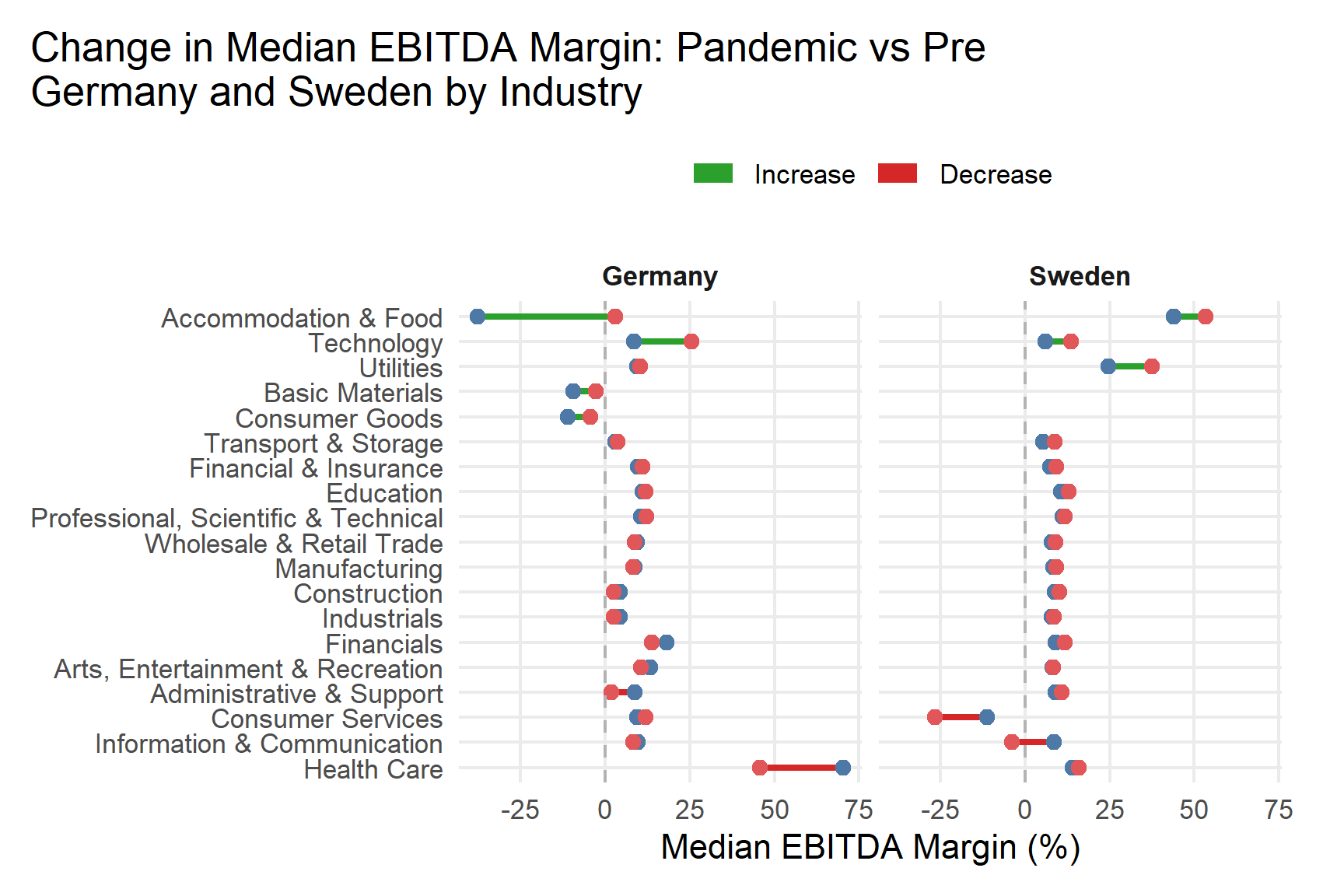
1. How did profitability change across industries?
This question investigates how profitability variables such as ROA, EBITDA margin, and EBIT margin shifted across industries between the pre-pandemic period (2018 to 2019) and the pandemic period (2020 to 2021) in Germany and Sweden. It aims to identify which sectors saw profit declines, remained stable, or grew during the pandemic. By comparing profitability trends across industries, the analysis highlights which sectors proved more resilient to the economic impacts of the pandemic. These insights help explain how the pandemic affected overall corporate performance and provide a clearer understanding of the differences in financial recovery among industries.
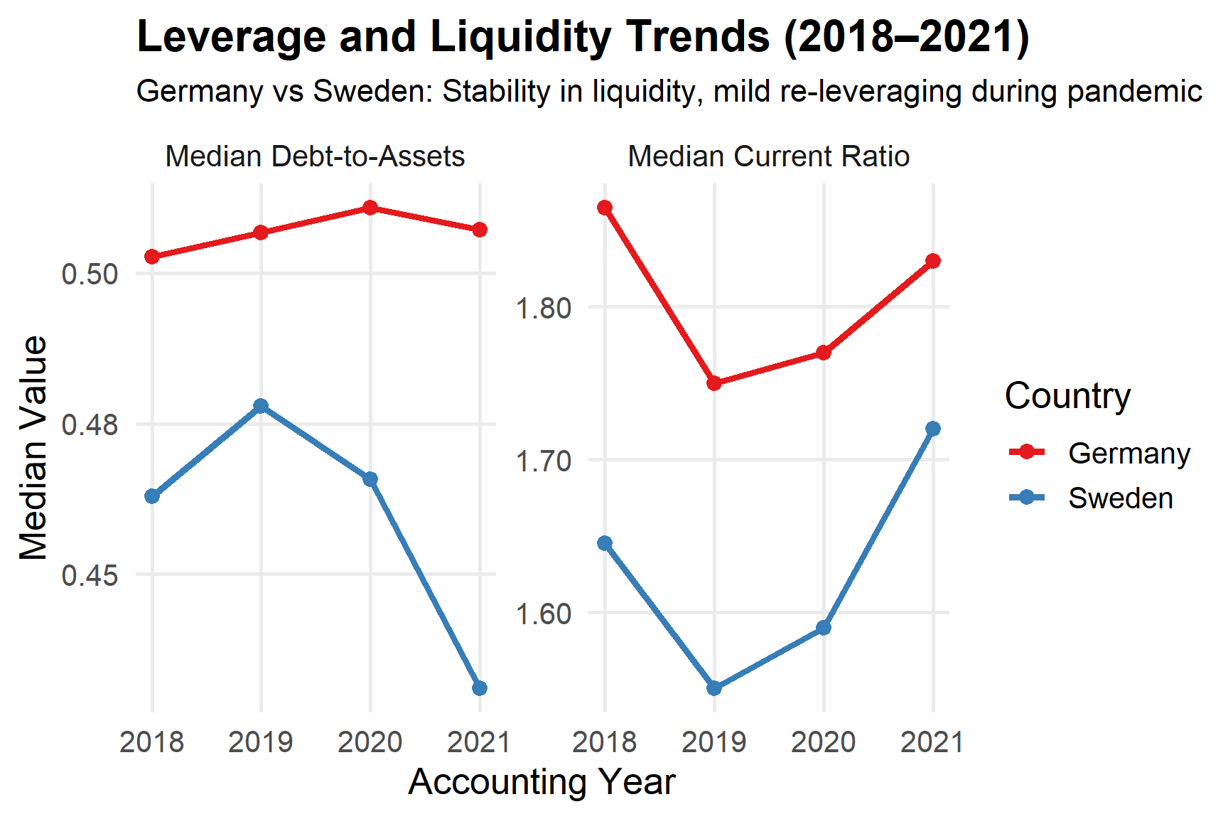
2. How did leverage (debt-to-assets) and liquidity (current ratio) evolve during pandemic?
This question extends the Part 1 analysis by comparing how leverage (debt-to-assets) and liquidity (current ratio) evolved between Germany and Sweden from 2018 to 2021.
The goal is to determine whether firms in the two economies displayed similar balance-sheet responses to the COVID-19 shock.
3. Which Sweden industries showed unexpected financial resilience or vulnerability from 2019 to 2021, and how were these outcomes shaped by profitability, leverage, liquidity, and firm size?
Between 2019 and 2021, Swedish industries showed mixed financial resilience. Manufacturing, IT, and professional services remained strong, maintaining profitability and liquidity despite the pandemic, helped by Sweden’s lighter restrictions and export strength. In contrast, hospitality, transport, and retail were more vulnerable, with sharp declines in profitability and higher leverage as firms relied on debt to survive. Larger firms recovered faster due to stronger cash reserves and financing access, while smaller firms faced liquidity pressures. Overall, industries with high profitability and low leverage before 2020 proved most resilient through 2021.
4. How did the fundamental relationship between corporate liquidity and profitability evolve and fracture within industries during the pandemic?
This study compares firms in Germany and Sweden, two advanced European economies with different financial systems and policy responses. The analysis explores how the ROA and CR relationship evolved and fractured within industries during and after the pandemic using time-series features and scagnostic metrics. ROA and Current Ratio reflect how efficiently firms generate profit and how safely they can cover short-term obligations. The goal is to reveal which sectors were most resilient, which experienced unequal recovery, and how national environments influenced these patterns. Understanding the changing relationship between ROA and CR can provide insight into the financial resilience of different industries. It also helps identify whether recovery followed a stable path or diverged into unequal outcomes, such as K-shaped patterns, where some firms recovered faster while others declined.
IDA
The Initial Data Analysis (IDA) evaluates data integrity, distributional behaviour, and comparability across Germany and Sweden before proceeding to substantive analysis.
Given that firm-level financial data are typically heavy-tailed, skewed, and heterogeneous across industries, this stage focuses on:
- Structural integrity of firm-year observations.
- Industry classification consistency.
- Distribution shape and outlier behaviour.
- Missingness patterns.
- Justification for robust summaries.
1. Structural Integrity and Missingness Checks
The first step standardises numeric fields, cleans text variables, reports missingness, and performs sanity checks for duplicates and impossible values.
Show code
num_cols <- c(
  "total_assets_eur","total_liabilities_eur","total_equity_eur",
  "total_revenue_eur","net_sales_eur","gross_sales_eur","net_income_eur",
  "ebit_margin_pct","ebitda_margin_pct","roa_pct","roe_pct",
  "net_assets_turnover","stock_turnover",
  "solvency_pct","gearing_pct","current_ratio","liquidity_ratio",
  "shareholders_liq_pct","interest_cover"
)

#symbol formatting/coerce numerics
filtered_germany_sweden <- filtered_germany_sweden |>
  mutate(
    across(all_of(num_cols) & where(is.character), readr::parse_number),
    country = stringr::str_to_title(country),
    city    = stringr::str_to_title(city)
  )

#missingness report check (overall and by year)
missing_overall <- filtered_germany_sweden |>
  summarise(across(everything(), ~ mean(is.na(.)))) |>
  pivot_longer(everything(), names_to = "variable", values_to = "missing_rate")

missing_by_year <- filtered_germany_sweden |>
  group_by(acct_year) |>
  summarise(across(everything(), ~ mean(is.na(.)))) |>
  pivot_longer(-acct_year, names_to = "variable", values_to = "missing_rate")

#sanity checks
dup_firm_year <- filtered_germany_sweden |>
  count(company_id, fy_year, acct_year, country) |>
  filter(n > 1)

impossible_assets <- filtered_germany_sweden |>
  filter(!is.na(total_assets_eur) & total_assets_eur < 0)

consol_levels <- filtered_germany_sweden |>
  count(consolidation_code, sort = TRUE)
This block confirms:
- Numeric variables are correctly parsed.
- Country and city labels are standardised.
- Duplicate firm-year records are absent.
- Impossible values (e.g., negative total assets) are flagged.
- Consolidation codes are reviewed.
Ensuring structural integrity at this stage prevents distortion in later cross-country comparisons.
2. Industry Classification Mapping
To enable consistent sector-level analysis, 2-digit NACE codes are extracted and mapped to broad industry groups. ICB classification is used as a fallback where necessary. A unified industry_group variable is then created.
Show code
#clean 2-digit NACE as integer
filtered_germany_sweden <- filtered_germany_sweden |>
  mutate(
    nace_num2 = suppressWarnings(as.integer(str_sub(readr::parse_number(as.character(nace_code)), 1, 2)))
  )

#map NACE divisions to broad section names
industry_from_nace <- function(x){
  case_when(
    x %in% 1:3 ~ "Agriculture, Forestry & Fishing",
    x %in% 5:9 ~ "Mining & Quarrying",
    x %in% 10:33 | x %in% 15:37 ~ "Manufacturing",
    x %in% 35 ~ "Electricity, Gas, Steam",
    x %in% 36:39 ~ "Water Supply & Waste",
    x %in% 41:43 ~ "Construction",
    x %in% 45:47 ~ "Wholesale & Retail Trade",
    x %in% 49:53 ~ "Transport & Storage",
    x %in% 55:56 ~ "Accommodation & Food",
    x %in% 58:63 ~ "Information & Communication",
    x %in% 64:66 ~ "Financial & Insurance",
    x %in% 68 ~ "Real Estate",
    x %in% 69:75 ~ "Professional, Scientific & Technical",
    x %in% 77:82 ~ "Administrative & Support",
    x %in% 84 ~ "Public Administration",
    x %in% 85 ~ "Education",
    x %in% 86:88 ~ "Human Health & Social Work",
    x %in% 90:93 ~ "Arts, Entertainment & Recreation",
    x %in% 94:96 ~ "Other Service Activities",
    x %in% 97:98 ~ "Household Activities",
    x %in% 99 ~ "Extraterritorial Organizations",
    TRUE ~ NA_character_
  )
}

#ICB top-level sector labels
icb_map <- c(
  "0001" = "Oil & Gas",
  "1000" = "Basic Materials",
  "2000" = "Industrials",
  "3000" = "Consumer Goods",
  "4000" = "Health Care",
  "5000" = "Consumer Services",
  "6000" = "Telecommunications",
  "7000" = "Utilities",
  "8000" = "Financials",
  "9000" = "Technology"
)

#normalize ICB to a 4-digit “bucket” (example: 2573 to 2000)
normalize_icb <- function(x){
  x_chr <- str_extract(as.character(x), "\\d+")
  ifelse(is.na(x_chr), NA_character_,
         sprintf("%04d", as.integer(floor(as.numeric(x_chr) / 1000) * 1000)))
}

filtered_germany_sweden <- filtered_germany_sweden |>
  mutate(
    industry_nace = industry_from_nace(nace_num2),
    icb_bucket    = normalize_icb(icb_code),
    industry_icb  = icb_map[icb_bucket],
    industry_group = coalesce(industry_nace, industry_icb, "Other / Unmapped")
  )

#check
unmapped_sample <- filtered_germany_sweden |>
  filter(industry_group == "Other / Unmapped") |>
  select(company_id, fy_year, acct_year, nace_code, icb_code) |>
  head(15)

#factor order for plots
ordered_levels <- c(
  "Agriculture, Forestry & Fishing","Mining & Quarrying","Manufacturing",
  "Electricity, Gas, Steam","Water Supply & Waste","Construction",
  "Wholesale & Retail Trade","Transport & Storage","Accommodation & Food",
  "Information & Communication","Financial & Insurance","Real Estate",
  "Professional, Scientific & Technical","Administrative & Support",
  "Public Administration","Education","Human Health & Social Work",
  "Arts, Entertainment & Recreation","Other Service Activities",
  "Household Activities","Extraterritorial Organizations",
  "Oil & Gas","Basic Materials","Industrials","Consumer Goods","Health Care",
  "Consumer Services","Telecommunications","Utilities","Financials","Technology",
  "Other / Unmapped"
)
filtered_germany_sweden <- filtered_germany_sweden |>
  mutate(industry_group = factor(industry_group, levels = ordered_levels))
This step ensures:
- Comparable industry groupings across Germany and Sweden.
- Reduced fragmentation from highly granular vendor codes.
- Consistent sector ordering for visualisation.
The mapping prioritises NACE classifications and supplements them with ICB where missing.
3. Reshaping for Distribution Profiling
Numeric variables are reshaped into long format to support systematic profiling. Variables are separated into:
- Scale variables (monetary totals).
- Ratio variables (profitability, liquidity, leverage).
Show code
#using long data
ida_germany_sweden <- filtered_germany_sweden |>
  dplyr::select(acct_year, country, dplyr::all_of(num_cols)) |>
  tidyr::pivot_longer(dplyr::all_of(num_cols),
                      names_to = "variable_orig", values_to = "value") |>
  tidyr::drop_na()

#split between scale and ratio
scale_vars <- c("total_assets_eur","total_liabilities_eur","total_equity_eur",
                "total_revenue_eur","net_sales_eur","gross_sales_eur","net_income_eur")
ratio_vars <- setdiff(unique(ida_germany_sweden$variable_orig), scale_vars)

#label mapping for the charts
nice <- c(
  total_assets_eur   = "Total assets (EUR)",
  total_liabilities_eur="Total liabilities (EUR)",
  total_equity_eur   = "Equity (EUR)",
  total_revenue_eur  = "Total revenue (EUR)",
  net_sales_eur      = "Net sales (EUR)",
  gross_sales_eur    = "Gross sales (EUR)",
  net_income_eur     = "Net income (EUR)",
  ebit_margin_pct    = "EBIT margin (%)",
  ebitda_margin_pct  = "EBITDA margin (%)",
  roa_pct            = "ROA (%)",
  roe_pct            = "ROE (%)",
  net_assets_turnover= "Net assets turnover (x)",
  stock_turnover     = "Stock turnover (x)",
  solvency_pct       = "Solvency (%)",
  gearing_pct        = "Gearing (%)",
  current_ratio      = "Current ratio (x)",
  liquidity_ratio    = "Liquidity ratio (x)",
  shareholders_liq_pct = "Shareholders’ liquidity (%)",
  interest_cover     = "Interest cover (x)"
)

pretty_var <- function(x) ifelse(x %in% names(nice), nice[x], x)

ida_germany_sweden <- ida_germany_sweden |>
  mutate(variable = pretty_var(variable_orig),
         variable = factor(variable, levels = unique(variable)))
Reshaping facilitates uniform treatment across variables and supports consistent visual diagnostics. Separating scale and ratio variables allows appropriate transformation choices (log scale for monetary values, linear scale for ratios).
Distributional Analysis
4. Scale Variables
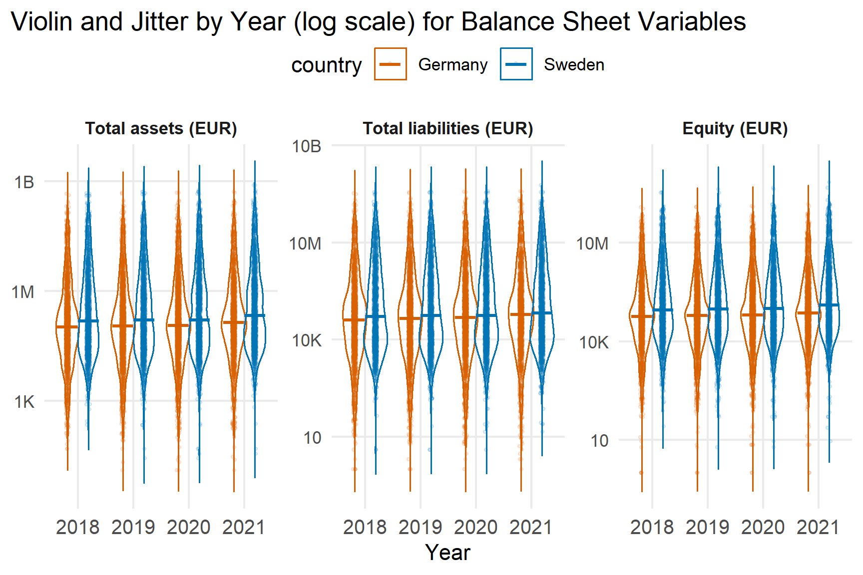
Scale variables are examined using violin and jitter plots on a log scale, with medians highlighted.
4.1 Variable Group Definitions
Show code
#define variables sets
vars_balance <- c("total_assets_eur","total_liabilities_eur","total_equity_eur")
vars_flows   <- c("total_revenue_eur","net_sales_eur","gross_sales_eur","net_income_eur")
This code defines balance-sheet and flow variable groups for visualisation.
4.2 Balanced Sheet Scale Variables
Show code
p_scale_balance <- ida_germany_sweden |>
  filter(variable_orig %in% vars_balance) |>
  mutate(
    y    = if_else(value > 0, value, NA_real_),
    year = factor(acct_year)
  ) |>
  ggplot(aes(x = year, y = y, colour = country,
             group = interaction(country, year))) +
  geom_violin(trim = FALSE, fill = NA, linewidth = 0.4, na.rm = TRUE,
              position = position_dodge(width = 0.75)) +
  geom_jitter(alpha = 0.12, size = 0.6, na.rm = TRUE,
              position = position_jitterdodge(jitter.width = 0.12,
                                              jitter.height = 0,
                                              dodge.width = 0.75)) +
  stat_summary(fun = median, geom = "point", shape = 95, size = 6, na.rm = TRUE,
               position = position_dodge(width = 0.75)) +
  scale_y_log10(labels = scales::label_number(scale_cut = scales::cut_short_scale())) +
  facet_wrap(~ variable, scales = "free_y", ncol = 3) +
  labs(x = "Year", y = NULL, title = "Violin and Jitter by Year (log scale) for Balance Sheet Variables") +
  theme_minimal(base_size = 11) +
  theme(
  plot.title.position = "plot",
  legend.position     = "top",
  legend.spacing.y    = unit(-0.6, "lines"),
  legend.justification = "center",
  legend.direction     = "horizontal",
  legend.box           = "horizontal",
  legend.margin        = margin(b = 4),
  axis.text.x          = element_text(size = 10),
  strip.text           = element_text(face = "bold"),
  panel.grid.minor     = element_blank()
)

p_scale_balance
Balance-sheet variables are strongly right-skewed in both countries. Most firms cluster at lower asset levels, while a small number of very large firms create long upper tails.
Key findings:
- Medians remain stable between 2018 and 2021.
- Sweden shows slightly higher central levels in asset and liability measures.
- Dispersion increases modestly during 2020 – 2021
The heavy skewness justifies the use of median and IQR rather than mean.
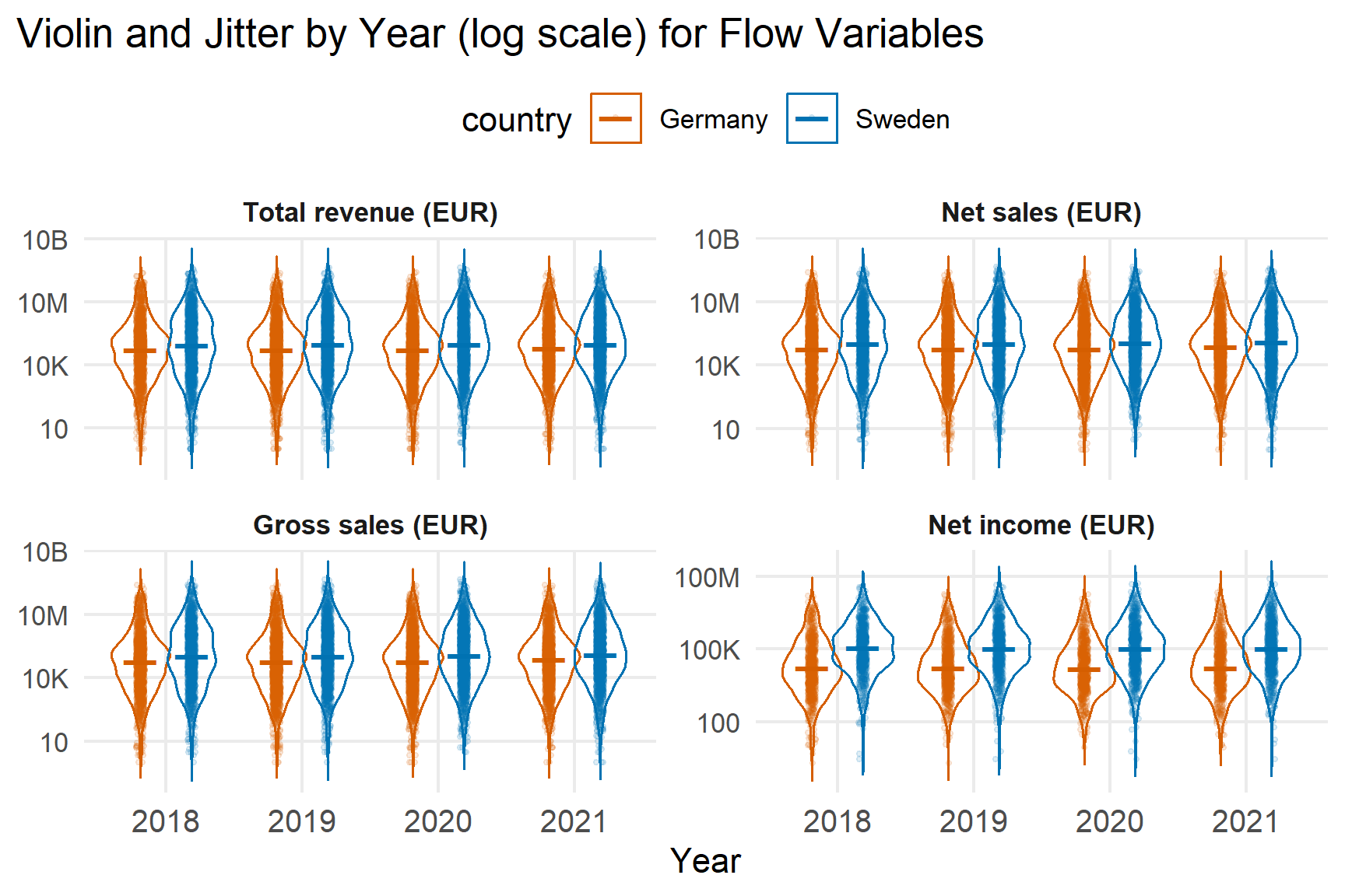
4.3 Flow Scale Variables
Show code
p_scale_flows <- ida_germany_sweden |>
  dplyr::filter(variable_orig %in% vars_flows) |>
  dplyr::mutate(
    y    = dplyr::if_else(value > 0, value, NA_real_),
    year = factor(acct_year)
  ) |>
  ggplot(aes(x = year, y = y, colour = country,
             group = interaction(country, year))) +
  geom_violin(trim = FALSE, fill = NA, linewidth = 0.4, na.rm = TRUE,
              position = position_dodge(width = 0.75)) +
  geom_jitter(alpha = 0.12, size = 0.6, na.rm = TRUE,
              position = position_jitterdodge(jitter.width = 0.12,
                                              jitter.height = 0,
                                              dodge.width = 0.75)) +
  stat_summary(fun = median, geom = "point", shape = 95, size = 6, na.rm = TRUE,
               position = position_dodge(width = 0.75)) +
  scale_y_log10(labels = scales::label_number(scale_cut = scales::cut_short_scale())) +
  facet_wrap(~ variable, scales = "free_y", ncol = 2) +
  labs(x = "Year", y = NULL, title = "Violin and Jitter by Year (log scale) for Flow Variables") +
  theme_minimal(base_size = 11) +
  theme(
  plot.title.position = "plot",
  legend.position     = "top",
  legend.spacing.y    = unit(0.3, "lines"),
  legend.justification = "center",
  legend.direction     = "horizontal",
  legend.box           = "horizontal",
  legend.margin        = margin(t = 6, b = 2),
  axis.text.x          = element_text(size = 10),
  strip.text           = element_text(face = "bold"),
  panel.grid.minor     = element_blank()
)

p_scale_flows
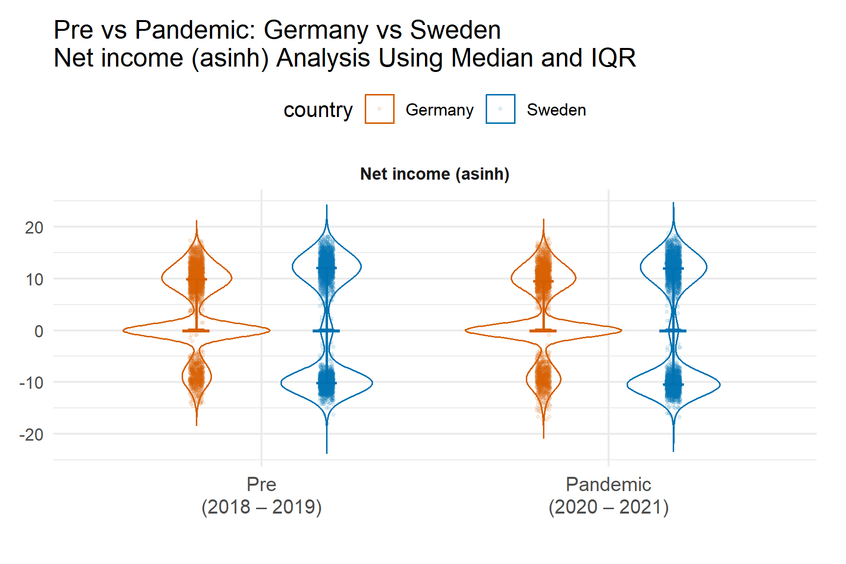
Revenue and sales measures show similar right-skewed distributions. Net income exhibits a thicker lower tail in 2020 – 2021, indicating increased incidence of low or negative profitability during the pandemic.
Again, medians provide a more robust summary than means.
5. Ratio Variables
Ratio variables are visualised on their natural scale to assess dispersion and potential structural shifts.
5.1 Variable Group Definitions
Show code
#define variable sets
vars_profit_eff <- c(
  "ebit_margin_pct", "ebitda_margin_pct",
  "roa_pct", "roe_pct",
  "net_assets_turnover", "stock_turnover"
)

vars_liquidity_solvency <- c(
  "solvency_pct", "gearing_pct",
  "current_ratio", "liquidity_ratio",
  "shareholders_liq_pct", "interest_cover"
)
This block defines profitability/efficiency and liquidity/solvency variable groups.
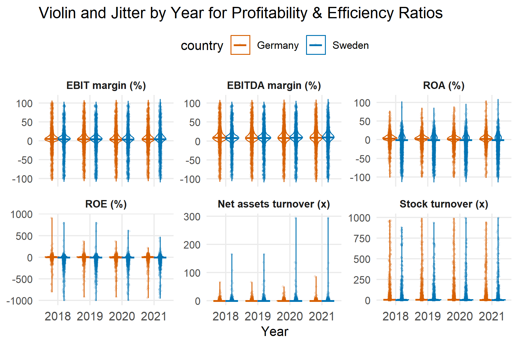
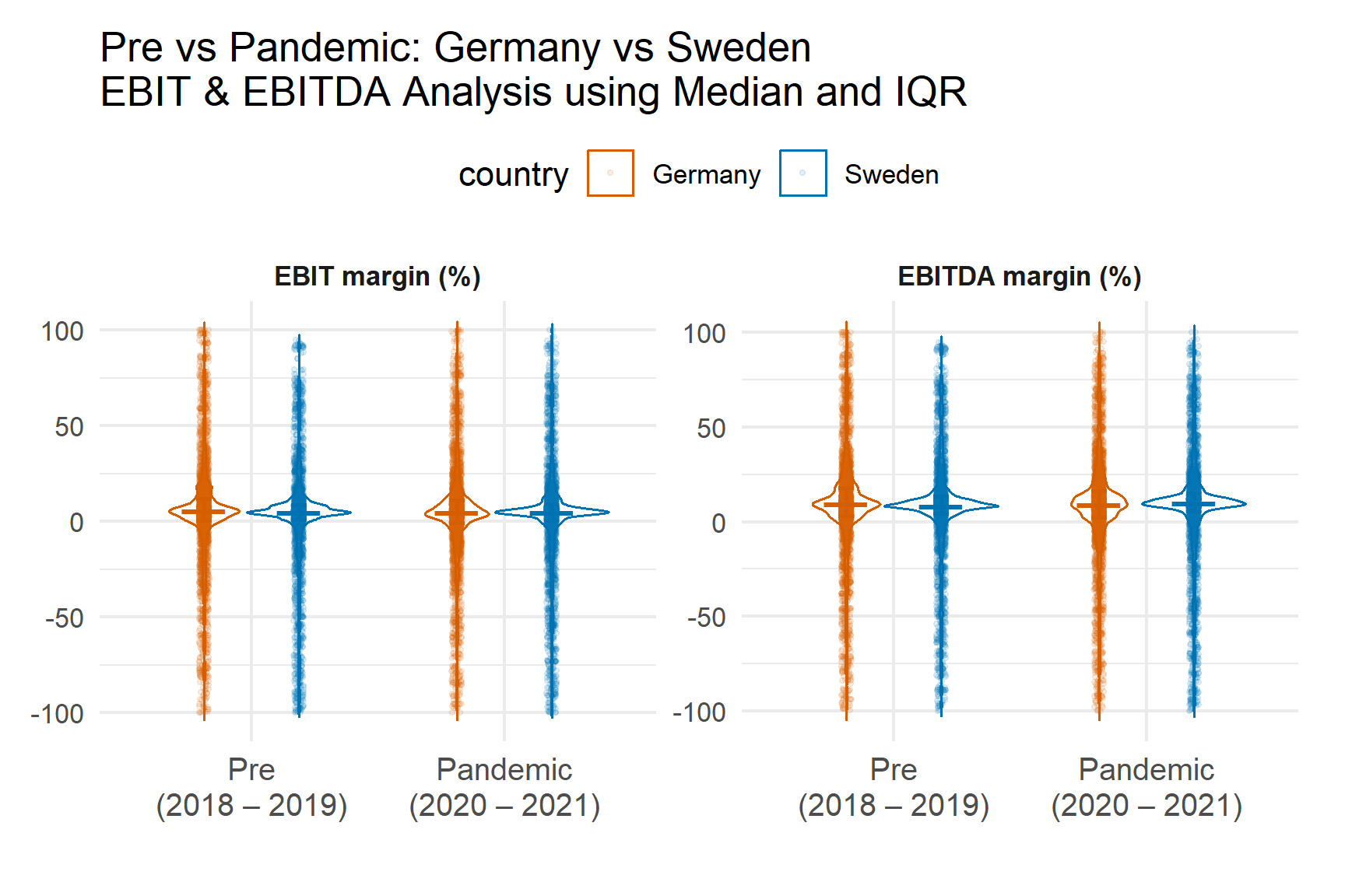
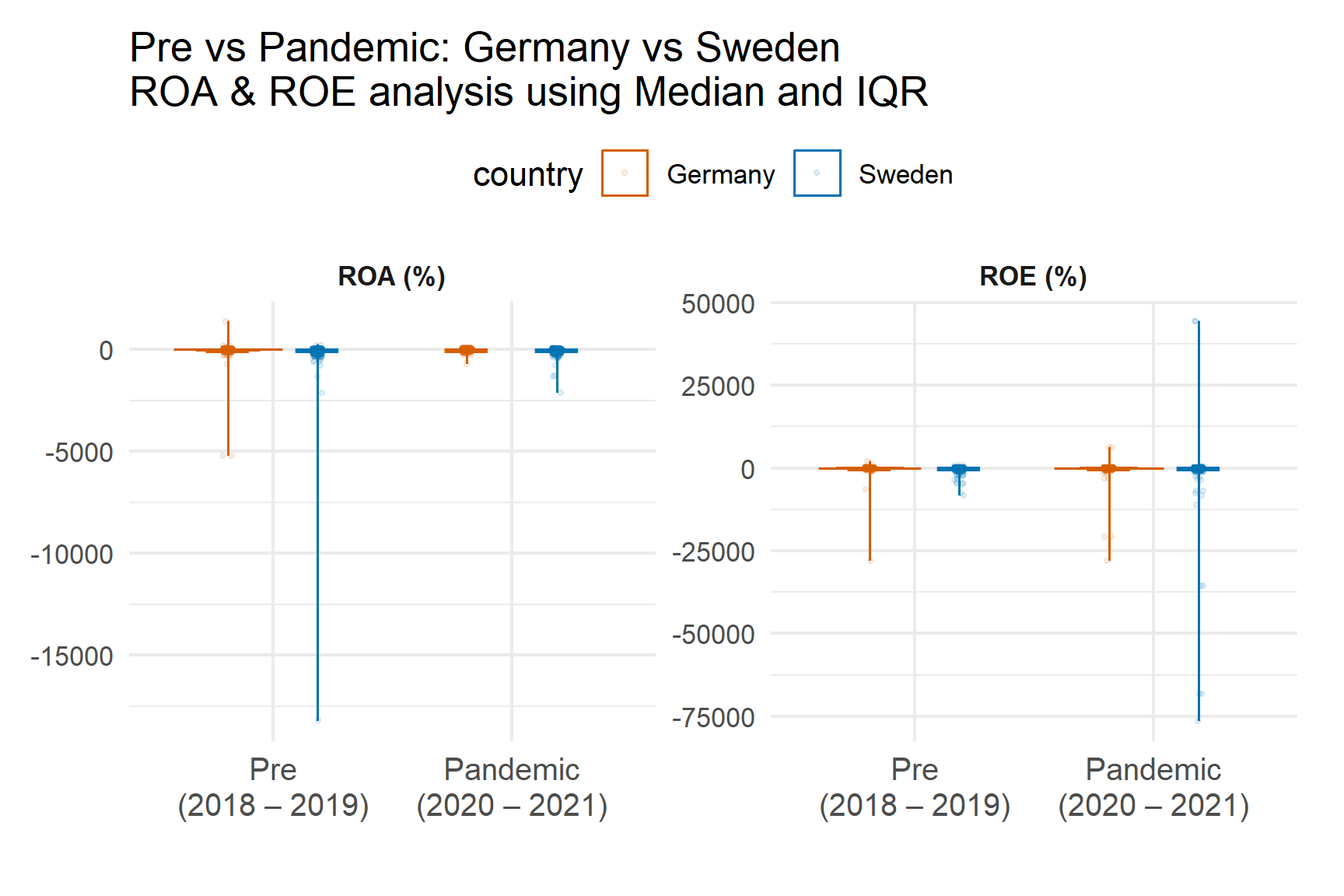
5.2 Profitability and Efficiency Ratios
Show code
p_ratio_profit_eff <- ida_germany_sweden |>
  dplyr::filter(variable_orig %in% vars_profit_eff) |>
  dplyr::mutate(year = factor(acct_year)) |>
  ggplot(aes(x = year, y = value, colour = country,
             group = interaction(country, year))) +
  geom_violin(trim = FALSE, fill = NA, linewidth = 0.4, na.rm = TRUE,
              position = position_dodge(width = 0.75)) +
  geom_jitter(alpha = 0.12, size = 0.6, na.rm = TRUE,
              position = position_jitterdodge(jitter.width = 0.12,
                                              jitter.height = 0,
                                              dodge.width = 0.75)) +
  stat_summary(fun = median, geom = "point",
               shape = 95, size = 6, na.rm = TRUE,
               position = position_dodge(width = 0.75)) +
  facet_wrap(~ variable, scales = "free_y", ncol = 3) +
  labs(x = "Year", y = NULL,
       title = "Violin and Jitter by Year for Profitability & Efficiency Ratios") +
  theme_minimal(base_size = 11) +
  theme(
    axis.text.x = element_text(size = 10),
    strip.text  = element_text(face = "bold"),
    panel.grid.minor = element_blank(),
    legend.position = "top"
  )

p_ratio_profit_eff
Profitability ratios cluster near zero but widen during the pandemic years. ROE displays the greatest dispersion, reflecting sensitivity to equity base fluctuations.
Efficiency ratios remain relatively stable, suggesting operational turnover was less volatile than bottom-line profitability.
Heavy tails confirm that median-based comparisons are appropriate.
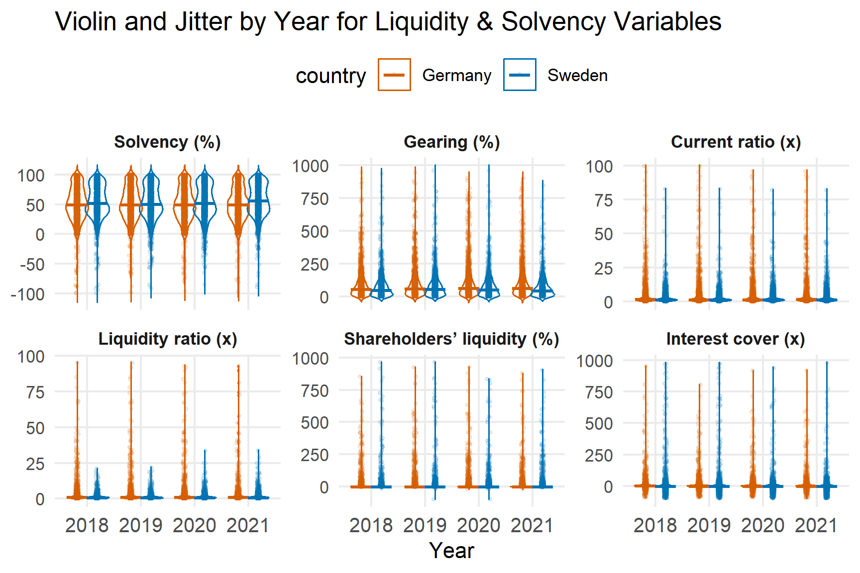
5.3 Liquidity and Solvency Ratios
Show code
p_ratio_liq_solv <- ida_germany_sweden |>
  dplyr::filter(variable_orig %in% vars_liquidity_solvency) |>
  dplyr::mutate(year = factor(acct_year)) |>
  ggplot(aes(x = year, y = value, colour = country,
             group = interaction(country, year))) +
  geom_violin(trim = FALSE, fill = NA, linewidth = 0.4, na.rm = TRUE,
              position = position_dodge(width = 0.75)) +
  geom_jitter(alpha = 0.12, size = 0.6, na.rm = TRUE,
              position = position_jitterdodge(jitter.width = 0.12,
                                              jitter.height = 0,
                                              dodge.width = 0.75)) +
  stat_summary(fun = median, geom = "point",
               shape = 95, size = 6, na.rm = TRUE,
               position = position_dodge(width = 0.75)) +
  facet_wrap(~ variable, scales = "free_y", ncol = 3) +
  labs(x = "Year", y = NULL,
       title = "Violin and Jitter by Year for Liquidity & Solvency Variables") +
  theme_minimal(base_size = 11) +
  theme(
    axis.text.x = element_text(size = 10),
    strip.text  = element_text(face = "bold"),
    panel.grid.minor = element_blank(),
    legend.position = "top"
  )

p_ratio_liq_solv
Liquidity measures are centred around operationally meaningful values, while gearing and interest coverage show long upper tails.
Sweden exhibits slightly greater dispersion across several ratios, consistent with earlier distributional findings.
Data Quality Diagnostics
6. Missingness Patterns
Missingness is examined by country and year.
Show code
key_vars <- c("total_assets_eur","total_liabilities_eur","total_equity_eur",
"total_revenue_eur","net_income_eur",
"ebit_margin_pct","ebitda_margin_pct","roa_pct","roe_pct",
"current_ratio","liquidity_ratio","gearing_pct","solvency_pct")
# missingness by industry and country
missing_by_industry <- filtered_germany_sweden |>
group_by(country, industry_group) |>
summarise(across(all_of(key_vars), ~ mean(is.na(.)), .names = "{.col}"),
.groups = "drop") |>
pivot_longer(-c(country, industry_group),
names_to = "variable", values_to = "missing_rate")
#heatmap by year for numeric variables
missing_heat <- filtered_germany_sweden |>
group_by(country, acct_year) |>
summarise(across(all_of(key_vars), ~ mean(is.na(.)), .names = "{.col}"),
.groups = "drop") |>
pivot_longer(-c(country, acct_year),
names_to = "variable", values_to = "missing_rate")
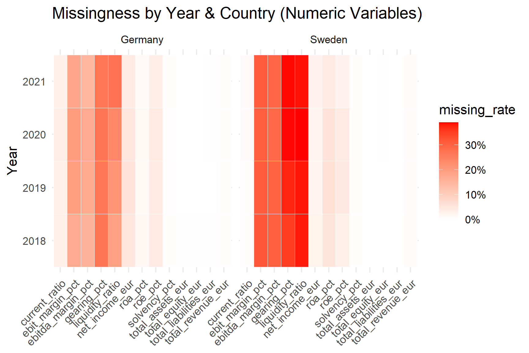
ggplot(missing_heat,
aes(variable, factor(acct_year), fill = missing_rate)) +
geom_tile(color = "white") +
scale_fill_gradient(low = "white", high = "red",
labels = scales::percent_format(accuracy = 1)) +
facet_wrap(~ country, nrow = 1) +
labs(x = NULL, y = "Year",
title = "Missingness by Year & Country (Numeric Variables)") +
theme_minimal() +
theme(axis.text.x = element_text(angle = 45, hjust = 1))
Missingness is stable across 2018–2021 and does not spike during the pandemic. Ratio variables (particularly gearing and liquidity ratio) exhibit higher missing rates than core accounting totals.
Balance-sheet and revenue variables are nearly complete, ensuring reliable cross-country comparisons for scale measures.
7. Outliers Detection
Outliers are flagged using both IQR (1.5× rule) and z-score thresholds.
Show code
num_cols <- c("total_assets_eur","total_liabilities_eur","total_equity_eur",
              "total_revenue_eur","net_sales_eur","gross_sales_eur","net_income_eur",
              "ebit_margin_pct","ebitda_margin_pct","roa_pct","roe_pct",
              "net_assets_turnover","stock_turnover",
              "solvency_pct","gearing_pct","current_ratio","liquidity_ratio",
              "shareholders_liq_pct","interest_cover")

qfun <- function(x,p) quantile(x, probs=p, na.rm=TRUE, names=FALSE)

outliers_by_country <- purrr::map_dfr(num_cols, function(v){
  x  <- filtered_germany_sweden[[v]]
  ct <- filtered_germany_sweden$country

  q1 <- qfun(x,.25); q3 <- qfun(x,.75); iqr <- q3-q1
  lo <- q1 - 1.5*iqr; hi <- q3 + 1.5*iqr
  z  <- as.numeric(scale(x))

  tibble::tibble(
    variable = v,
    country  = ct,
    n        = !is.na(x),
    iqr_flag = (x < lo | x > hi),
    z_flag   = abs(z) > 3
  )
}) |>
  dplyr::group_by(variable, country) |>
  dplyr::summarise(
    n = sum(n),
    iqr_outliers = sum(iqr_flag, na.rm = TRUE),
    z_outliers   = sum(z_flag, na.rm = TRUE),
    share_iqr    = iqr_outliers/n,
    share_z      = z_outliers/n,
    .groups = "drop"
  ) |>
  dplyr::arrange(country, desc(share_iqr))

var_levels <- intersect(num_cols, unique(outliers_by_country$variable))

outliers_by_country_ord <- outliers_by_country |>
  dplyr::mutate(variable = factor(variable, levels = var_levels)) |>
  dplyr::arrange(variable, country)

outliers_by_country_ord |>
  kable(align = "l", booktabs = TRUE) |>
  kable_styling(full_width = FALSE, font_size = 11)
| total_assets_eur |
Germany |
8042 |
1117 |
57 |
0.14 |
0.01 |
| total_assets_eur |
Sweden |
7150 |
1451 |
145 |
0.20 |
0.02 |
| total_liabilities_eur |
Germany |
8038 |
1201 |
60 |
0.15 |
0.01 |
| total_liabilities_eur |
Sweden |
7150 |
1483 |
100 |
0.21 |
0.01 |
| total_equity_eur |
Germany |
8041 |
1070 |
38 |
0.13 |
0.00 |
| total_equity_eur |
Sweden |
7146 |
1482 |
145 |
0.21 |
0.02 |
| total_revenue_eur |
Germany |
8003 |
1045 |
79 |
0.13 |
0.01 |
| total_revenue_eur |
Sweden |
7094 |
1584 |
132 |
0.22 |
0.02 |
| net_sales_eur |
Germany |
7909 |
1028 |
79 |
0.13 |
0.01 |
| net_sales_eur |
Sweden |
7018 |
1581 |
132 |
0.23 |
0.02 |
| gross_sales_eur |
Germany |
7909 |
1033 |
77 |
0.13 |
0.01 |
| gross_sales_eur |
Sweden |
7013 |
1580 |
132 |
0.23 |
0.02 |
| net_income_eur |
Germany |
7643 |
1052 |
32 |
0.14 |
0.00 |
| net_income_eur |
Sweden |
6980 |
2404 |
131 |
0.34 |
0.02 |
| ebit_margin_pct |
Germany |
6554 |
1179 |
90 |
0.18 |
0.01 |
| ebit_margin_pct |
Sweden |
4920 |
1183 |
101 |
0.24 |
0.02 |
| ebitda_margin_pct |
Germany |
6736 |
1170 |
77 |
0.17 |
0.01 |
| ebitda_margin_pct |
Sweden |
5024 |
1079 |
92 |
0.21 |
0.02 |
| roa_pct |
Germany |
7938 |
391 |
83 |
0.05 |
0.01 |
| roa_pct |
Sweden |
6754 |
1344 |
270 |
0.20 |
0.04 |
| roe_pct |
Germany |
7717 |
468 |
81 |
0.06 |
0.01 |
| roe_pct |
Sweden |
6885 |
1317 |
226 |
0.19 |
0.03 |
| net_assets_turnover |
Germany |
7953 |
351 |
26 |
0.04 |
0.00 |
| net_assets_turnover |
Sweden |
6990 |
568 |
61 |
0.08 |
0.01 |
| stock_turnover |
Germany |
4859 |
962 |
171 |
0.20 |
0.04 |
| stock_turnover |
Sweden |
4178 |
617 |
86 |
0.15 |
0.02 |
| solvency_pct |
Germany |
8018 |
70 |
67 |
0.01 |
0.01 |
| solvency_pct |
Sweden |
7113 |
71 |
57 |
0.01 |
0.01 |
| gearing_pct |
Germany |
5891 |
517 |
183 |
0.09 |
0.03 |
| gearing_pct |
Sweden |
4457 |
213 |
75 |
0.05 |
0.02 |
| current_ratio |
Germany |
7786 |
989 |
237 |
0.13 |
0.03 |
| current_ratio |
Sweden |
7097 |
704 |
66 |
0.10 |
0.01 |
| liquidity_ratio |
Germany |
6217 |
794 |
178 |
0.13 |
0.03 |
| liquidity_ratio |
Sweden |
4394 |
356 |
10 |
0.08 |
0.00 |
| shareholders_liq_pct |
Germany |
7912 |
1166 |
150 |
0.15 |
0.02 |
| shareholders_liq_pct |
Sweden |
5632 |
1002 |
110 |
0.18 |
0.02 |
| interest_cover |
Germany |
7089 |
1014 |
108 |
0.14 |
0.02 |
| interest_cover |
Sweden |
5543 |
1394 |
128 |
0.25 |
0.02 |
Outliers are common in scale variables due to heterogeneous firm size. Profitability ratios also show extreme values, particularly ROE.
These patterns confirm:
- Heavy-tailed distributions.
- Need for robust summaries.
- Potential benefit of log transformations for monetary variables.
No automatic winsorisation is applied at this stage; instead, robustness is addressed in later modelling decisions.
8. Character Field Validation
Key identifiers and classification fields are cleaned and checked for missingness.
Show code
#character variables to check
char_vars <- c("company_id","company_name","country","city",
               "consolidation_code","nace_code","icb_code","sic_code")
char_vars <- intersect(char_vars, names(filtered_germany_sweden))

#cleaning
chars_clean <- filtered_germany_sweden |>
  mutate(
    across(all_of(char_vars),
           ~ .x |> as.character() |> str_squish() |> na_if("")),
    #casing
    country = str_to_title(country),
    city    = str_to_title(city),
    company_name = str_squish(company_name)
  )

#missingness check
char_missing <- chars_clean |>
  summarise(across(all_of(char_vars), ~ mean(is.na(.)))) |>
  tidyr::pivot_longer(everything(), names_to="variable", values_to="missing_rate")

char_missing |>
  kable(align = "l", booktabs = TRUE) |>
  kable_styling(full_width = FALSE, font_size = 11)
| company_id |
0.00 |
| company_name |
0.00 |
| country |
0.00 |
| city |
0.00 |
| consolidation_code |
0.00 |
| nace_code |
0.02 |
| icb_code |
0.09 |
| sic_code |
0.00 |
Identifiers (company_id, company_name) are complete, enabling reliable panel tracking. Industry codes are largely complete, supporting consistent classification.
After completing the global IDA, targeted preparation steps were applied for each research question.
Question 1
I initially added a period label (Pre-pandemic 2018 – 2019 vs. Pandemic 2020 – 2021). For visualisations, net_income_eur was transformed using asinh() to compare both gains and losses on a consistent scale. When ROA/ROE are missing, I recalculated simple estimates from the accounting totals and noted the sources of the values (reported vs. recomputed).
Show code
stopifnot("net_income_eur" %in% names(filtered_germany_sweden))

ida_question1 <- filtered_germany_sweden |>
  mutate(
    country = country,
    # period flag
    period = if_else(acct_year >= 2020, "Pandemic (2020–2021)", "Pre-pandemic (2018–2019)"),
    # transform for visuals (handles negatives)
    net_income_eur_asinh = asinh(as.numeric(net_income_eur)),
    # recompute ROA / ROE (fallbacks)
    roa_calc = 100 * (net_income_eur / total_assets_eur),
    roe_calc = if_else(total_equity_eur > 0,
                       100 * (net_income_eur / total_equity_eur),
                       NA_real_),
    roa_use = coalesce(roa_pct, roa_calc),
    roe_use = coalesce(roe_pct, roe_calc),
    roa_src = case_when(
      !is.na(roa_pct) ~ "reported",
      !is.na(roa_calc) ~ "recomputed",
      TRUE ~ NA_character_
    ),
    roe_src = case_when(
      !is.na(roe_pct) ~ "reported",
      !is.na(roe_calc) ~ "recomputed",
      TRUE ~ NA_character_
    )
  )
This step:
- Defines pre-pandemic vs pandemic periods
- Transforms net income using asinh() to handle losses
- Recomputes ROA and ROE when missing
- Tracks provenance of values
This ensures transparency in profitability construction.
Conservative Within-firm Gap Filling
Show code
#Firm one-gap fill within the same period only

fill_one_gap <- function(x){
  f <- dplyr::lag(x); b <- dplyr::lead(x)
  ifelse(is.na(x) & !is.na(f) & !is.na(b) & (f == b), f, x)
}

ida_question1 <- ida_question1 |>
  arrange(company_id, acct_year) |>
  group_by(company_id, period) |>  #period boundary blocks carryover
  mutate(
    ebit_step1   = fill_one_gap(ebit_margin_pct),
    ebitda_step1 = fill_one_gap(ebitda_margin_pct),
    roa_step1    = fill_one_gap(roa_use),
    roe_step1    = fill_one_gap(roe_use)
  ) |>
  ungroup() |>
  mutate(
    ebit_step1   = coalesce(ebit_margin_pct, ebit_step1),
    ebitda_step1 = coalesce(ebitda_margin_pct, ebitda_step1),
    roa_step1    = coalesce(roa_use, roa_step1),
    roe_step1    = coalesce(roe_use, roe_step1)
  )
A one-gap rule fills isolated missing values within the same period only, preventing cross-period information leakage.
Hierarchical Median Imputation
Show code
#median fills in strict order (no cross-period borrowing)
#country x industry × year medians
med_ixy <- ida_question1 |>
  group_by(country, industry_group, acct_year) |>
  summarise(
    med_ebit = median(ebit_step1,   na.rm=TRUE),
    med_ebitda = median(ebitda_step1, na.rm=TRUE),
    med_roa = median(roa_step1,    na.rm=TRUE),
    med_roe = median(roe_step1,    na.rm=TRUE),
    .groups="drop"
  )

#country x industry × period medians
med_ip <- ida_question1 |>
  group_by(country, industry_group, period) |>
  summarise(
    med_ebit_ip = median(ebit_step1,   na.rm=TRUE),
    med_ebitda_ip = median(ebitda_step1, na.rm=TRUE),
    med_roa_ip = median(roa_step1,    na.rm=TRUE),
    med_roe_ip = median(roe_step1,    na.rm=TRUE),
    .groups="drop"
  )

#country x period medians
med_p <- ida_question1 |>
  group_by(country, period) |>
  summarise(
    med_ebit_p = median(ebit_step1,   na.rm=TRUE),
    med_ebitda_p = median(ebitda_step1, na.rm=TRUE),
    med_roa_p = median(roa_step1,    na.rm=TRUE),
    med_roe_p = median(roe_step1,    na.rm=TRUE),
    .groups="drop"
  )

#join and impute with precedence, also explicit source flags
ida_question1 <- ida_question1 |>
  left_join(med_ixy, by = c("country","industry_group","acct_year")) |>
  left_join(med_ip,  by = c("country","industry_group","period")) |>
  left_join(med_p,   by = c("country", "period")) |>
  mutate(
    #final values, using your precedence
    ebit_margin_q1   = if_else(is.na(ebitda_step1), ebit_step1, ebit_step1),
    ebit_margin_q1   = if_else(is.na(ebit_step1),   coalesce(med_ebit,   med_ebit_ip,   med_ebit_p),   ebit_step1),
    ebitda_margin_q1 = if_else(is.na(ebitda_step1), coalesce(med_ebitda, med_ebitda_ip, med_ebitda_p), ebitda_step1),
    roa_q1           = if_else(is.na(roa_step1),    coalesce(med_roa,    med_roa_ip,    med_roa_p),    roa_step1),
    roe_q1           = if_else(is.na(roe_step1),    coalesce(med_roe,    med_roe_ip,    med_roe_p),    roe_step1),

    #provenance for EBIT/EBITDA margins
    ebit_src = dplyr::case_when(
      !is.na(ebit_margin_pct) ~ "reported",
      is.na(ebit_margin_pct) & !is.na(ebit_step1) ~ "firm-1gap(period)",
      is.na(ebit_step1) & !is.na(med_ebit) ~ "ind×year",
      is.na(ebit_step1) & is.na(med_ebit) & !is.na(med_ebit_ip) ~ "ind×period",
      TRUE ~ "period"
    ),
    ebitda_src = dplyr::case_when(
      !is.na(ebitda_margin_pct) ~ "reported",
      is.na(ebitda_margin_pct) & !is.na(ebitda_step1) ~ "firm-1gap(period)",
      is.na(ebitda_step1) & !is.na(med_ebitda) ~ "ind×year",
      is.na(ebitda_step1) & is.na(med_ebitda) & !is.na(med_ebitda_ip) ~ "ind×period",
      TRUE ~ "period"
    ),

    #ROA/ROE provenance
    roa_src = dplyr::case_when(
      !is.na(roa_src) ~ roa_src,
      is.na(roa_src) & !is.na(roa_step1) ~ "firm-1gap(period)",
      is.na(roa_step1) & !is.na(med_roa) ~ "ind×year",
      is.na(roa_step1) & is.na(med_roa) & !is.na(med_roa_ip) ~ "ind×period",
      TRUE ~ "period"
    ),
    roe_src = dplyr::case_when(
      !is.na(roe_src) ~ roe_src,
      is.na(roe_src) & !is.na(roe_step1) ~ "firm-1gap(period)",
      is.na(roe_step1) & !is.na(med_roe) ~ "ind×year",
      is.na(roe_step1) & is.na(med_roe) & !is.na(med_roe_ip) ~ "ind×period",
      TRUE ~ "period"
    )
  ) |>
  select(-ends_with("_step1"))
Remaining gaps are filled using a strict hierarchy:
- Country × Industry × Year median.
- Country × Industry × Period median.
- Country × Period median.
All imputation sources are explicitly recorded.
Imputation Audit Tables
Show code
impute_summary_q1 <- ida_question1 |>
  summarise(
    .by = c(country, period),
    n_rows = n(),
    ebit_reported   = sum(ebit_src   == "reported",            na.rm=TRUE),
    ebit_firmgap    = sum(ebit_src   == "firm-1gap(period)",   na.rm=TRUE),
    ebit_ind_year   = sum(ebit_src   == "ind×year",            na.rm=TRUE),
    ebit_ind_period = sum(ebit_src   == "ind×period",          na.rm=TRUE),
    ebit_period     = sum(ebit_src   == "period",              na.rm=TRUE),

    ebitda_reported   = sum(ebitda_src   == "reported",          na.rm=TRUE),
    ebitda_firmgap    = sum(ebitda_src   == "firm-1gap(period)", na.rm=TRUE),
    ebitda_ind_year   = sum(ebitda_src   == "ind×year",          na.rm=TRUE),
    ebitda_ind_period = sum(ebitda_src   == "ind×period",        na.rm=TRUE),
    ebitda_period     = sum(ebitda_src   == "period",            na.rm=TRUE),

    roa_reported    = sum(roa_src == "reported",            na.rm=TRUE),
    roa_recomputed  = sum(roa_src == "recomputed",          na.rm=TRUE),
    roa_firmgap     = sum(roa_src == "firm-1gap(period)",   na.rm=TRUE),
    roa_ind_year    = sum(roa_src == "ind×year",            na.rm=TRUE),
    roa_ind_period  = sum(roa_src == "ind×period",          na.rm=TRUE),
    roa_period      = sum(roa_src == "period",              na.rm=TRUE),

    roe_reported    = sum(roe_src == "reported",            na.rm=TRUE),
    roe_recomputed  = sum(roe_src == "recomputed",          na.rm=TRUE),
    roe_firmgap     = sum(roe_src == "firm-1gap(period)",   na.rm=TRUE),
    roe_ind_year    = sum(roe_src == "ind×year",            na.rm=TRUE),
    roe_ind_period  = sum(roe_src == "ind×period",          na.rm=TRUE),
    roe_period      = sum(roe_src == "period",              na.rm=TRUE)
  )
Imputation rates remain limited. Germany shows higher direct reporting coverage than Sweden, particularly for EBIT and EBITDA margins. ROA and ROE are largely reported in both countries.
- EBIT & EBITDA Imputation
Show code
impute_margins <- impute_summary_q1 |>
  select(country, period, n_rows,
         ebit_reported, ebit_ind_year, ebit_period, ebit_firmgap,
         ebitda_reported, ebitda_ind_year, ebitda_period, ebitda_firmgap)

impute_margins |>
  kable(align = "l", booktabs = TRUE) |>
  kable_styling(full_width = FALSE, font_size = 11)
| Germany |
Pre-pandemic (2018–2019) |
4071 |
3326 |
745 |
0 |
0 |
3399 |
672 |
0 |
0 |
| Germany |
Pandemic (2020–2021) |
3975 |
3228 |
747 |
0 |
0 |
3337 |
638 |
0 |
0 |
| Sweden |
Pre-pandemic (2018–2019) |
3477 |
2384 |
1089 |
4 |
0 |
2427 |
1046 |
4 |
0 |
| Sweden |
Pandemic (2020–2021) |
3675 |
2536 |
1135 |
4 |
0 |
2597 |
1073 |
4 |
1 |
According to the table, Germany shows strong coverage of EBIT and EBITDA margins in both periods, with about 82 – 84% of values reported directly. The remaining 16 – 18% are filled using industry and year medians, and Germany does not need any firm-gap or period-level imputations. In comparison, Sweden has lower direct reporting, around 69 – 71% across both periods. Approximately 29 – 31% of Swedish records depend on industry and year medians, which is a higher dependence than in Germany. Only four rows in each period use a period-level fallback, indicating that heavy imputations are very limited. Overall, imputations are present in both countries, but Sweden requires more support due to lower direct reporting.
- ROA Imputation
Show code
impute_roa <- impute_summary_q1 |>
  select(country, period, n_rows,
         roa_reported, roa_recomputed, roa_ind_year, roa_ind_period, roa_period)

impute_roa |>
  kable(align = "l", booktabs = TRUE) |>
  kable_styling(full_width = FALSE, font_size = 11)
| Germany |
Pre-pandemic (2018–2019) |
4071 |
4008 |
52 |
11 |
0 |
0 |
| Germany |
Pandemic (2020–2021) |
3975 |
3930 |
43 |
2 |
0 |
0 |
| Sweden |
Pre-pandemic (2018–2019) |
3477 |
3269 |
201 |
7 |
0 |
0 |
| Sweden |
Pandemic (2020–2021) |
3675 |
3485 |
179 |
10 |
0 |
0 |
According to the table, ROA is nearly fully available in Germany, with 98 – 99% of rows reported directly in both periods. Only about 1% of observations depend on recomputation from accounting totals, and industry and year replacement is below 0.3%. Sweden also shows strong ROA coverage, around 94 – 95% reported or recomputed. However, Sweden relies more on recomputation, approximately 5% in each period. Industry-level fallback is very limited. Overall, data quality remains stable in both countries, though Sweden requires slightly more reconstruction of ROA than Germany.
- ROE Imputation
Show code
impute_roe <- impute_summary_q1 |>
  select(country, period, n_rows,
         roe_reported, roe_recomputed, roe_ind_year, roe_ind_period, roe_period)

impute_roe |>
  kable(align = "l", booktabs = TRUE) |>
  kable_styling(full_width = FALSE, font_size = 11)
| Germany |
Pre-pandemic (2018–2019) |
4071 |
3902 |
16 |
153 |
0 |
0 |
| Germany |
Pandemic (2020–2021) |
3975 |
3815 |
18 |
142 |
0 |
0 |
| Sweden |
Pre-pandemic (2018–2019) |
3477 |
3339 |
37 |
101 |
0 |
0 |
| Sweden |
Pandemic (2020–2021) |
3675 |
3546 |
27 |
102 |
0 |
0 |
According to the table, Germany had strong ROE availability, with about 96% of records reported directly in both periods. Around 0.4 – 0.5% were recomputed, and roughly 3 – 4% used industry and year fallbacks. Sweden also had good coverage, above 94% reported in both periods. However, Sweden relied more on recomputation and on industry and year fallbacks combined, accounting for around 5 – 6% of observations. No period-level imputations occurred in either country. Overall, both datasets provided reliable ROE values, with Sweden needing slightly more support from industry medians.
The relatively high direct reporting coverage in Germany compared to Sweden suggests stronger raw data completeness, although both datasets remain sufficiently robust for comparative analysis. Importantly, the imputation hierarchy preserves cross-country comparability while minimising distortion from extreme firm-level observations.
Question 2
The Initial Data Analysis (IDA) for this question focused on constructing and validating key indicators of leverage and liquidity for both Germany and Sweden during 2018 – 2021. Specifically, new variables such as debt-to-assets and equity ratio were derived from total liabilities, equity, and assets to measure firms’ capital structure and solvency capacity. Data cleaning steps included filtering out inactive firms, excluding implausible ratios (e.g., leverage >150%), and dropping missing or non-finite values. These processed metrics were summarised using median and interquartile range (IQR) to capture typical firm behaviour and variability by year and country, ensuring comparability between economies before conducting visual exploration.
Show code
# Create leverage and liquidity indicators for both countries
lev_liq_data <- filtered_germany_sweden |>
  filter(acct_year %in% 2018:2021, status == "Active") |>
  mutate(
    debt_to_assets = total_liabilities_eur / total_assets_eur,
    equity_ratio   = total_equity_eur / total_assets_eur
  ) |>
  select(acct_year, country, industry_group,
         debt_to_assets, equity_ratio, gearing_pct,
         solvency_pct, current_ratio) |>
  drop_na(debt_to_assets, current_ratio)

# Summarise by year and country
lev_liq_summary <- lev_liq_data |>
  group_by(country, acct_year) |>
  summarise(
    median_debt_assets = median(debt_to_assets, na.rm = TRUE),
    iqr_debt_assets    = IQR(debt_to_assets, na.rm = TRUE),
    median_liquidity   = median(current_ratio, na.rm = TRUE),
    iqr_liquidity      = IQR(current_ratio, na.rm = TRUE),
    .groups = "drop"
  )

lev_liq_summary |>
  knitr::kable(
    caption = "Median and IQR of Leverage and Liquidity by Country (2018–2021)",
    digits = 2
  ) |>
  kableExtra::kable_styling(full_width = FALSE, font_size = 11)
Median and IQR of Leverage and Liquidity by Country (2018–2021)
| Germany |
2018 |
0.50 |
0.37 |
1.9 |
2.6 |
| Germany |
2019 |
0.51 |
0.38 |
1.8 |
2.5 |
| Germany |
2020 |
0.51 |
0.38 |
1.8 |
2.5 |
| Germany |
2021 |
0.51 |
0.37 |
1.8 |
2.4 |
| Sweden |
2018 |
0.46 |
0.40 |
1.6 |
2.2 |
| Sweden |
2019 |
0.48 |
0.40 |
1.6 |
1.9 |
| Sweden |
2020 |
0.47 |
0.41 |
1.6 |
2.1 |
| Sweden |
2021 |
0.43 |
0.40 |
1.7 |
2.7 |
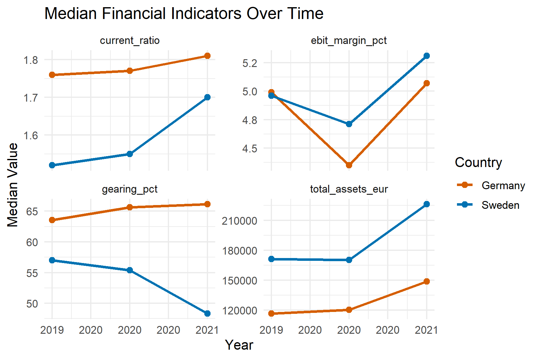
Both countries maintained median liquidity near 1.8×, while median leverage hovered around 0.50-0.52.Sweden shows slightly higher liquidity dispersion, suggesting a broader mix of firm sizes and capital structures.
The stability of median leverage during 2020 – 2021 indicates that firms did not materially increase debt exposure despite favourable credit conditions. This suggests that pandemic-related stress manifested more through profitability pressures than through widespread balance-sheet deterioration.
Question 3
- Financial Indicators Summaries
Show code
industry_financial_summary <- filtered_germany_sweden |>
  filter(country == "Germany", !is.na(industry_group), acct_year >= 2019, acct_year <= 2021) |>
  mutate(period = ifelse(acct_year < 2020, "Pre-pandemic", "Pandemic")) |>
  group_by(industry_group, period) |>
  summarise(
    n_firms = n(),
    median_profit = median(net_income_eur, na.rm = TRUE),
    median_roa = median(roa_pct, na.rm = TRUE),
    median_liq = median(current_ratio, na.rm = TRUE),
    median_lev = median(gearing_pct, na.rm = TRUE),
    .groups = "drop"
  ) |>
  arrange(industry_group, period)

# Display table
knitr::kable(
  industry_financial_summary,
  digits = 2,
  booktabs = TRUE,
  caption = "Industry-level summary as per IDA procedure"
)
Industry-level summary as per IDA procedure
| Manufacturing |
Pandemic |
1690 |
0 |
2.48 |
1.91 |
64.4 |
| Manufacturing |
Pre-pandemic |
893 |
0 |
3.84 |
1.94 |
64.4 |
| Construction |
Pandemic |
7 |
94700 |
5.33 |
0.95 |
144.1 |
| Construction |
Pre-pandemic |
4 |
54500 |
7.48 |
1.04 |
98.1 |
| Wholesale & Retail Trade |
Pandemic |
43 |
6200 |
5.19 |
1.43 |
81.2 |
| Wholesale & Retail Trade |
Pre-pandemic |
22 |
1400 |
4.91 |
1.60 |
81.2 |
| Transport & Storage |
Pandemic |
273 |
0 |
2.61 |
1.62 |
71.2 |
| Transport & Storage |
Pre-pandemic |
142 |
0 |
2.37 |
1.74 |
49.5 |
| Accommodation & Food |
Pandemic |
13 |
-18900 |
-3.18 |
1.79 |
34.9 |
| Accommodation & Food |
Pre-pandemic |
10 |
0 |
-4.78 |
1.79 |
54.2 |
| Information & Communication |
Pandemic |
120 |
0 |
2.58 |
1.28 |
99.4 |
| Information & Communication |
Pre-pandemic |
75 |
381 |
4.22 |
1.41 |
117.9 |
| Financial & Insurance |
Pandemic |
149 |
0 |
3.28 |
1.46 |
70.2 |
| Financial & Insurance |
Pre-pandemic |
79 |
0 |
1.60 |
1.43 |
74.2 |
| Professional, Scientific & Technical |
Pandemic |
873 |
0 |
3.65 |
1.84 |
72.4 |
| Professional, Scientific & Technical |
Pre-pandemic |
463 |
0 |
3.88 |
1.67 |
73.9 |
| Administrative & Support |
Pandemic |
8 |
0 |
-3.14 |
1.71 |
21.9 |
| Administrative & Support |
Pre-pandemic |
3 |
106 |
11.78 |
3.34 |
45.9 |
| Education |
Pandemic |
58 |
0 |
0.26 |
1.41 |
52.6 |
| Education |
Pre-pandemic |
31 |
0 |
3.34 |
1.97 |
46.4 |
| Arts, Entertainment & Recreation |
Pandemic |
163 |
0 |
0.00 |
0.97 |
38.3 |
| Arts, Entertainment & Recreation |
Pre-pandemic |
88 |
0 |
1.92 |
1.20 |
29.2 |
| Basic Materials |
Pandemic |
6 |
-596 |
-14.53 |
0.85 |
15.4 |
| Basic Materials |
Pre-pandemic |
4 |
-801 |
-16.47 |
0.72 |
29.2 |
| Industrials |
Pandemic |
53 |
0 |
-1.58 |
2.00 |
67.2 |
| Industrials |
Pre-pandemic |
25 |
0 |
-0.17 |
2.51 |
40.6 |
| Consumer Goods |
Pandemic |
8 |
-32 |
-6.03 |
0.86 |
55.9 |
| Consumer Goods |
Pre-pandemic |
4 |
-32 |
-6.22 |
NA |
NA |
| Health Care |
Pandemic |
6 |
-638 |
-2.19 |
25.58 |
NA |
| Health Care |
Pre-pandemic |
4 |
-638 |
-2.47 |
2.23 |
NA |
| Consumer Services |
Pandemic |
10 |
0 |
-1.30 |
1.77 |
28.3 |
| Consumer Services |
Pre-pandemic |
8 |
0 |
-3.34 |
0.48 |
41.6 |
| Utilities |
Pandemic |
63 |
34573 |
2.29 |
1.07 |
176.8 |
| Utilities |
Pre-pandemic |
36 |
0 |
2.21 |
1.15 |
161.2 |
| Financials |
Pandemic |
354 |
0 |
1.96 |
2.42 |
42.8 |
| Financials |
Pre-pandemic |
192 |
0 |
2.10 |
2.21 |
34.0 |
| Technology |
Pandemic |
14 |
902 |
0.34 |
5.30 |
1.0 |
| Technology |
Pre-pandemic |
13 |
509 |
0.50 |
4.31 |
2.2 |
| Other / Unmapped |
Pandemic |
64 |
0 |
-2.09 |
1.45 |
29.3 |
| Other / Unmapped |
Pre-pandemic |
33 |
0 |
0.00 |
1.55 |
50.2 |
This code generates an industry-level summary of key financial indicators for German firms from 2019 – 2021, distinguishing between pre-pandemic and pandemic periods. It calculates the median values of profitability, ROA, liquidity, and leverage for each industry group, ensuring robustness against outliers. The resulting summary enables comparison of financial performance across industries, highlighting shifts in profitability and stability during the pandemic.
- Outlier Detection (IQR Rule)
Show code
outlier_summary <- function(x) {
  q1 <- quantile(x, 0.25, na.rm=TRUE)
  q3 <- quantile(x, 0.75, na.rm=TRUE)
  iqr <- q3 - q1
  lower <- q1 - 1.5 * iqr
  upper <- q3 + 1.5 * iqr
  sum(x < lower | x > upper, na.rm=TRUE)
}
financial_vars <- c("ebit_margin_pct", "gearing_pct", "current_ratio", "total_assets_eur")
outlier_counts_sweden <- filtered_germany_sweden  |>
  filter(country == "Sweden", acct_year >= 2019, acct_year <= 2021)  |>
  summarise(across(all_of(financial_vars), outlier_summary))

knitr::kable(outlier_counts_sweden, caption="Outlier counts for Sweden: Key financial variables (IQR rule)")
Outlier counts for Sweden: Key financial variables (IQR rule)
| 808 |
180 |
602 |
973 |
This code applies the Interquartile Range (IQR) rule to detect outliers among key financial variables for Swedish firms between 2019 and 2021. For each variable, EBIT margin, gearing ratio, current ratio, and total assets, the function calculates the first (Q1) and third (Q3) quartiles, determines the IQR, and identifies values lying beyond 1.5×IQR from these bounds as outliers. The resulting table reports the count of extreme observations per variable. This method provides a robust, non-parametric approach to identifying unusually high or low financial values, which helps assess data quality, detect potential anomalies, and ensure the reliability of subsequent statistical analyses.
- Data Completeness
Show code
# Prepare long-format data (already done)
missing_long_compare <- filtered_germany_sweden |>
filter(country %in% c("Sweden", "Germany"), acct_year >= 2018, acct_year <= 2021) |>
select(country, acct_year, all_of(financial_vars)) |>
pivot_longer(-c(country, acct_year), names_to = "variable", values_to = "value") |>
mutate(missing = is.na(value)) |>
group_by(country, acct_year, variable) |>
summarise(prop_missing = mean(missing), .groups = "drop")
# Ribbon plot
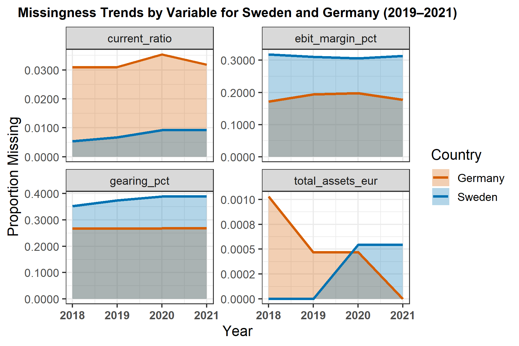
ggplot(missing_long_compare, aes(x = acct_year, y = prop_missing, fill = country, group = country)) +
geom_ribbon(aes(ymin = 0, ymax = prop_missing), alpha = 0.3) +
geom_line(aes(color = country), size = 1) +
facet_wrap(~variable, scales = "free_y") +
labs(
title = "Missingness Trends by Variable for Sweden and Germany (2019–2021)",
x = "Year",
y = "Proportion Missing",
fill = "Country",
color = "Country"
) +
scale_y_continuous(labels = function(x) sprintf("%.4f", x)) +
theme_bw(base_size = 12) +
theme(
plot.title = element_text(face = "bold", hjust = 0.5, size = 11),
axis.text.x = element_text(face = "bold"),
legend.position = "right"
)
This plot visualizes data completeness across key financial variables for Sweden and Germany between 2018 and 2021. It shows the proportion of missing values for each variable and year, allowing a direct comparison of data quality between the two countries. The ribbon and line format highlights both the level and trend of missingness over time. Consistently low proportions indicate reliable data coverage, while noticeable peaks suggest potential data reporting or collection gaps. Overall, this visualization supports a systematic evaluation of data integrity, ensuring that subsequent analyses are based on robust and complete financial information.
- Comparative Summary Table: Germany vs Sweden (Pandemic Years)
Show code
combined_financial_summary <- filtered_germany_sweden  |>
  filter(country %in% c("Germany", "Sweden"), !is.na(industry_group), acct_year >= 2019, acct_year <= 2021)  |>
  group_by(country, industry_group)  |>
  summarise(
    median_roa = median(roa_pct, na.rm = TRUE),
    median_liq = median(current_ratio, na.rm = TRUE),
    median_lev = median(gearing_pct, na.rm = TRUE)
  )  |>
  pivot_wider(names_from = country, values_from = c(median_roa, median_liq, median_lev))

knitr::kable(combined_financial_summary,
             digits = 2,
             booktabs = TRUE,
             caption = "Comparison of Key Financial Medians by Industry: Germany vs Sweden (2019-2021)")
Comparison of Key Financial Medians by Industry: Germany vs Sweden (2019-2021)
| Manufacturing |
3.11 |
-5.17 |
1.92 |
1.95 |
64.4 |
47.2 |
| Construction |
6.27 |
-40.70 |
1.01 |
1.17 |
124.4 |
28.8 |
| Wholesale & Retail Trade |
5.19 |
5.82 |
1.49 |
1.35 |
81.2 |
79.6 |
| Transport & Storage |
2.52 |
-2.34 |
1.62 |
1.71 |
62.6 |
52.5 |
| Accommodation & Food |
-3.94 |
4.57 |
1.79 |
0.52 |
50.0 |
7.5 |
| Information & Communication |
3.08 |
-6.38 |
1.31 |
0.79 |
102.9 |
218.9 |
| Financial & Insurance |
3.13 |
0.05 |
1.45 |
1.14 |
72.8 |
44.5 |
| Professional, Scientific & Technical |
3.76 |
2.91 |
1.79 |
1.30 |
73.1 |
65.5 |
| Administrative & Support |
-2.07 |
5.83 |
1.98 |
0.90 |
21.9 |
176.7 |
| Education |
2.76 |
-3.85 |
1.93 |
1.46 |
52.6 |
44.8 |
| Arts, Entertainment & Recreation |
0.16 |
-4.85 |
1.07 |
1.00 |
35.5 |
62.0 |
| Basic Materials |
-15.81 |
NA |
0.85 |
NA |
29.2 |
NA |
| Industrials |
-0.32 |
-7.09 |
2.04 |
1.80 |
61.6 |
72.6 |
| Consumer Goods |
-6.12 |
NA |
0.86 |
NA |
55.9 |
NA |
| Health Care |
-2.47 |
7.58 |
15.53 |
1.01 |
NA |
63.4 |
| Consumer Services |
-2.18 |
-24.76 |
1.38 |
1.09 |
34.8 |
1.3 |
| Utilities |
2.29 |
4.60 |
1.08 |
1.18 |
168.3 |
93.8 |
| Financials |
2.05 |
3.54 |
2.31 |
3.45 |
40.1 |
20.4 |
| Technology |
0.34 |
5.41 |
4.31 |
2.98 |
1.6 |
19.0 |
| Other / Unmapped |
-1.36 |
-1.46 |
1.45 |
2.33 |
46.4 |
99.3 |
This comparative summary table presents the median financial indicators, return on assets (ROA), liquidity (current ratio), and leverage (gearing), for Germany and Sweden across various industries during the pandemic period (2019 – 2021). By summarizing and contrasting these median values, the table highlights cross-country differences in financial performance and stability at the industry level. For instance, higher median liquidity in one country may reflect stronger short-term solvency, while lower leverage suggests more conservative financing structures. Overall, this table provides a concise yet informative overview of how the two economies’ industries responded financially during the pandemic years, enabling targeted comparisons of resilience and financial health.
These sectoral differences indicate that financial resilience was shaped primarily by pre-pandemic capital structure and profitability levels rather than by uniform macroeconomic shock effects. The pandemic therefore amplified existing structural strengths and weaknesses across industries.
Question 4
- Data Cleaning on Consolidation Codes
The raw data from Orbis contained financial statements under different consolidation codes (C1, C2, C*, U1, U2). To ensure consistency and comparability, we prioritized consolidated accounts which represent the entire economic entity. For each firm-year observation, we retained the highest-priority available consolidated statement following the order: C1 > C2 > C*. Unconsolidated statements (U1, U2) were excluded from the analysis.
Show code
ger_swe_q4 <- filtered_germany_sweden |>
  mutate(
    consolidation_priority = case_when(
      consolidation_code == "C1" ~ 1,  # highest priority
      consolidation_code == "C2" ~ 2,
      consolidation_code == "C*" ~ 3,
      consolidation_code == "U1" ~ 99, # Very low priority, about to be filtered
      consolidation_code == "U2" ~ 99,
      TRUE ~ 99  # Handle any unexpected code
    )
  ) |>

  # Group by company and year, and keep only the highest priority records
  group_by(company_id, fy_year) |>
  arrange(consolidation_priority, .by_group = TRUE) |>
  slice(1) |> # Take the first row of each group, which has the highest priority
  ungroup() |>
  # Filter out the remaining non-consolidated records
  filter(consolidation_priority %in% c(1, 2, 3))
- Select the columns to be analyzed
Show code
ger_swe_q4 <- ger_swe_q4 |>
  select(company_id, fy_year, roa_pct, current_ratio, industry_group, country)
The analysis in this study is based on a dataset of company financial information. It is important to note that in this question we use the fiscal year, not the calendar year. A company’s fiscal year is its own 12-month reporting period, which may not end in December. Using the fiscal year is more accurate for this research because it matches the company’s true business cycle. This means that when we refer to “2020” in the data, we are talking about the fiscal year that was most affected by the pandemic, even if it does not exactly match the calendar year 2020.
- Convert data into a tsibble object using the tsibble package
Each company was defined as a key and the financial year as the index. Basic screening was performed to check for missing values, outliers, and duplicates.
Show code
ger_swe_ts <- ger_swe_q4 |>
  as_tsibble(key = company_id, index = fy_year) |>
  arrange(company_id, fy_year)
- Missing value - Check for missing value
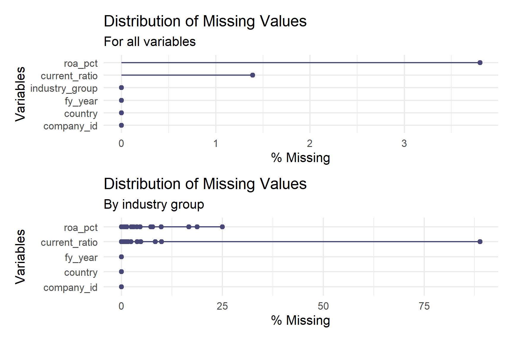
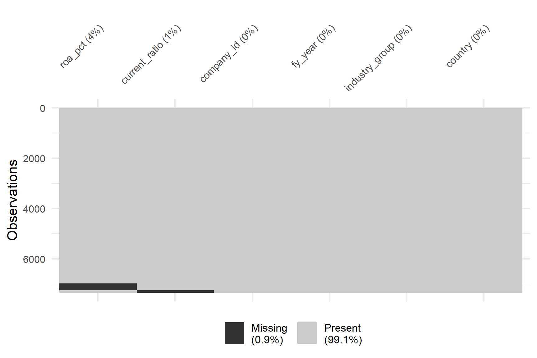
The initial examination of missing values revealed a relatively low proportion of incomplete data in the dataset. As shown in Figure 2, the missing value analysis showed that only 0.9% of the total data was missing, while 99.1% of observations were complete. ROA contained between 3% and 3.5% missing values across the dataset, while the current ratio had a slightly higher proportion of missing data, ranging from 1% to 2% (Figure 1).
Show code
# Check for missing ROA and CR
miss_var <-
  gg_miss_var(ger_swe_ts, show_pct = TRUE) +
  labs(title = "Distribution of Missing Values",
       subtitle = "For all variables")

# Check for missing values by industry group
miss_industry <- ger_swe_ts |>
  group_by(industry_group) |>
  gg_miss_var(show_pct = TRUE) +
  labs(title = "Distribution of Missing Values",
       subtitle = "By industry group")


miss_var / miss_industry
Show code
m3 <- vis_miss(ger_swe_ts, cluster = TRUE, sort_miss = TRUE) +
  theme(axis.text.x = element_text(size = 8, angle = 45, hjust = 1),
        axis.text.y = element_text(size = 8))

m3
Address missingness issues
To address missing data, observations with missing values in either ROA or current ratio were removed from the dataset. Additionally, to ensure temporal consistency across the study period, only industry groups that contained data for all three years (2019 – 2021) were retained. The ‘Other / Unmapped’ category was removed from the study as it comprises companies without clear industry classification.
Show code
ger_swe_ts <- ger_swe_ts |>
  as_tibble() |>   # Convert to a normal tibble
  # Remove observations with missing ROA or CR
  filter(!is.na(roa_pct) & !is.na(current_ratio)) |>
   # Remove industries that don't have data in 2019-2021
  group_by(industry_group) |>
  filter(all(2019:2021 %in% fy_year)) |>
  filter(industry_group != "Other / Unmapped") |>
  ungroup() |>
  # Convert back to tsibble format
  as_tsibble(key = company_id, index = fy_year) |>
  arrange(company_id, fy_year)
- Summary
The data preparation followed the same cleaning and preprocessing pipeline as described for Germany, ensuring comparability across the two countries. Consolidated financial statements were prioritized, and only industries with complete data for 2019 – 2021 were retained.
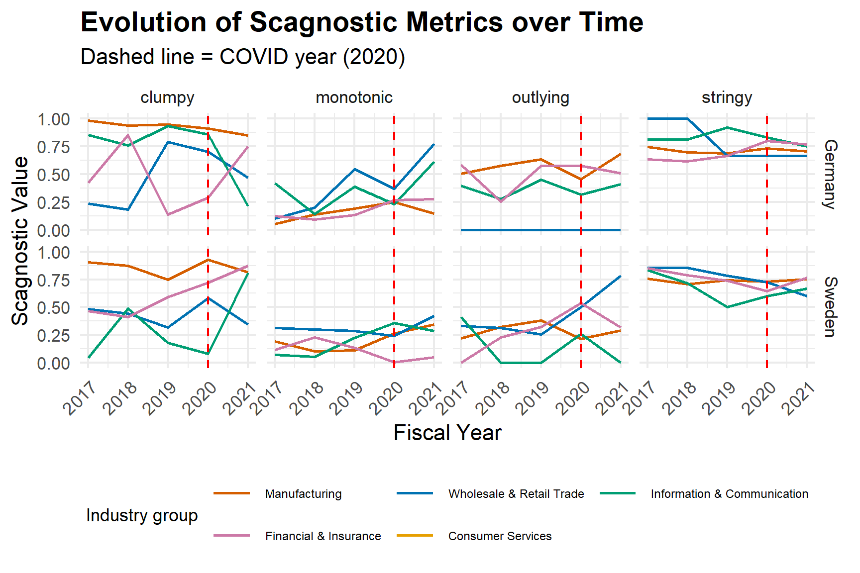
The comparative analysis of ROA and Current Ratio trends (Table 1) from 2017 to 2021 reveals stark differences between Germany and Sweden, with distinct pandemic-related patterns. German companies demonstrated remarkable resilience in profitability, with ROA recovering strongly from a low of 0.37% in 2020 to peak at 5.00% in 2021. It indicates a robust post-pandemic recovery. In contrast, Swedish firms maintained consistently negative ROA throughout the period, ranging from -9.69% to -11.29%. It suggests persistent profitability challenges unaffected by the pandemic. Regarding liquidity, both countries maintained stable Current Ratios. German companies showed more volatility, dipping to 2.62 in 2019 before recovering to 3.11 in 2020. However, Swedish firms maintained consistently higher ratios between 2.95-3.48, indicating stronger short-term liquidity positions.
This difference suggests that while the pandemic significantly impacted German profitability with a subsequent strong recovery, Swedish companies faced deeper structural profitability issues. But both maintained adequate short-term financial stability throughout the period.
Show code
kable(ger_swe_ts |>
  as_tibble() |>
  group_by(fy_year, country) |>
  summarise(mean_roa = mean(roa_pct, na.rm = TRUE),
            mean_cr = mean(current_ratio, na.rm = TRUE)) |>
  ungroup())
The divergence between profitability and liquidity patterns suggests that firms prioritised short-term financial buffers even when profitability weakened. This decoupling highlights an adaptive balance-sheet response rather than a simultaneous collapse in operational and liquidity conditions.
Summary per Question
Question 1
The analysis indicates that overall profitability remained broadly stable in both Germany and Sweden during the pandemic relative to the pre-pandemic period. Median EBIT, EBITDA, ROA, ROE, and net income stayed close to zero, suggesting that the typical firm did not experience a structural collapse in profitability.
However, dispersion increased during 2020–2021, particularly in Sweden, where firms experienced more extreme positive and negative outcomes. At the industry level, most sectors showed only modest changes in median EBITDA margins. Accommodation and Food recorded the strongest rebound, while Health Care experienced the largest decline. Technology, Utilities, and Education remained comparatively stable in both countries.
These findings suggest that the pandemic did not dramatically shift central profitability trends, but it amplified heterogeneity across firms and industries, especially within service-oriented sectors.
Question 2
Both Germany and Sweden displayed financial resilience during the COVID-19 period, though through different balance sheet adjustments.
Liquidity levels remained stable in both countries, with current ratios around 1.8 to 1.9. This indicates effective short-term financial management throughout the crisis. Sweden exhibited slightly greater dispersion, reflecting more variation in firm size and funding structures.
Leverage increased moderately in 2020 in both economies. German firms relied more heavily on external borrowing, consistent with strong credit support mechanisms. Swedish firms appear to have relied more on internal liquidity buffers.
The negative relationship between leverage and solvency is evident in both countries, though the steeper slope in Germany suggests greater sensitivity to debt accumulation. Industry patterns are broadly similar, with Manufacturing, Transport, and Construction remaining more leveraged, while Information, Health Care, and Professional Services maintain more conservative capital structures.
Overall, German firms’ solvency was more exposed to leverage increases, while Swedish firms’ diversified financial structures supported steadier post-pandemic adjustment.
Question 3
The comparative analysis of Germany and Sweden between 2019 and 2021 reveals distinct resilience patterns during the pandemic.
Both countries experienced profitability pressures and balance sheet adjustments. However, Swedish firms maintained more stable median profitability and liquidity, with fewer extreme outliers. German firms exhibited greater cross-industry variation, particularly in hospitality and transport, indicating more uneven financial stress.
These results suggest that Sweden’s corporate sector adapted with smoother financial adjustment, while Germany experienced sharper disruptions across certain industries, alongside recovery signals in capital-intensive sectors.
Question 4
The pandemic altered not only financial performance levels but also the structural relationship between liquidity and profitability.
Macro-level analysis shows that Germany maintained relatively stable trend strength and contained volatility across industries. Sweden displayed stronger fluctuations and more frequent structural breakdown in the profitability–liquidity relationship.
Micro-level scagnostic analysis reinforces this contrast. Swedish industries experienced larger increases in clustering, outliers, and residual dispersion, indicating stronger firm-level divergence. Germany showed comparatively steadier slope evolution and more consistent financial alignment.
The evidence suggests that Germany’s institutional environment supported stability in liquidity management, while Sweden’s more flexible structure allowed greater dispersion in firm outcomes. In several sectors, particularly Information and Communication, this resulted in K-shaped recovery dynamics.
Overall, resilience during the pandemic depended not only on firm-level financial management but also on national institutional and policy environments shaping adjustment mechanisms.